Category Hydrosystems Engineering Reliability Assessment and Risk Analysis

The antithetic-variates technique (Hammersley and Morton, 1956) achieves the variance-reduction goal by attempting to generate random variates that would induce a negative correlation for the quantity of interest between separate sim­ulation runs. Consider that Gq and ©2 are two unbiased estimators of an un­known quantity в to be estimated. The two estimators can be combined together to form another estimator as

1

G a = 2(®1 + ®2)

The new estimator Ga also is unbiased and has a variance as

Var(©a) = 1 [Var(©1) + Var(©2) + 2Cov(©b ©2)] 4

If the two estimators ©1 and ©2 were computed by Monte Carlo simulation through generating two independent, sets of random variates, they would be independent, and the variance for ©a would be

Var(© a) = 1[Var(©i) + Var©)] (6.77)

4

From Eq. (6.76) one realizes that the variance associated with ©a could be reduced if the Monte Carlo simulation can generate random variates, which result in a strong negative correlation between ©1 and ©2.

In a Monte Carlo simulation, the values of estimators ©1 and ©2 are functions of the generated random variates, which, in turn, are related to the standard uniform random variates. Therefore, ©1 and ©2 are functions of the two stan­dard uniform random variables U1 and U2. The objective to produce negative Cov[©©1(U1), ©2(U2)] can be achieved by producing U1 and U2, which are nega­tively correlated. However, it would not be desirable to complicate the computa­tional procedure by generating two sets of uniform random variates subject to the constraint of being negatively correlated. One simple approach to generate negatively correlated uniform random variates with minimal computation is to let U1 = 1 — U2. It can be shown that Cov(U, 1-U) = -1/12 (see Problem 6.31). Hence a simple antithetic-variates algorithm is the following:

1. Generate ui from U(0, 1), and compute 1 – ui, for i = 1, 2,…, n.

2. Compute 91(ui), 02(1 – ui), and then Qa according to Eq. (6.75).

Example 6.10 Develop a Monte Carlo algorithm using the antithetic-variates tech­nique to evaluate the integral G defined by

b

g (x) dx

in which g (x) is a given function.

Solution Applying the Monte Carlo method to estimate the value of G, the preceding integral can be rewritten as

where fx(x) is the adopted distribution function based on which random variates are generated. As can be seen, the original integral becomes the calculation of the expectation of the ratio of g (X) and fx(X). Hence the two estimators for G using the antithetic-variates technique can be formulated as

G = ьА g( X 1i)

1 n^fx ( X 1i)

i=1

G = 1 V g(X2i)

2 n f x (X2i)

i = 1

in which Xa = F-l(Ui) and X2i = F—1(1 — Ui), with Fx(■) being the CDF of the random variable X. The algorithm for the Monte Carlo integral using the antithetic – variates technique is

1. Generate n uniform random variates Ui from U(0, 1), and compute the correspond­ing 1 — Ui.

2. Compute g(xu), fx(X1i), g(X2i), and fx(X2i), with xu = F—1(ui) and X2i =

F—l(1 — ui).

3. Calculate the values of G1 and G2 by Eqs. (6.78a) and (6.78b), respectively. Then estimate G by Ga = (G1 + G2V2.

In the case that X has a uniform distribution as fx(x) = 1/(b — a), a < x < b, the estimate of G by the antithetic-variates technique can be expressed as

b — n

ga = ^na ^2g(x1i) + g(x2i)] (6.79)

i=1

Rubinstein (1981) showed that the antithetic-variates estimator, in fact, is more ef­ficient if g (x) is a continuous monotonically increasing or decreasing function with continuous first derivatives.

Example 6.11 Referring to pump reliability Example 6.6, estimate the pump fail­ure probability using the antithetic-variates technique along with the sample-mean Monte Carlo algorithm with n = 1000. The PDF selected is a uniform distribu­tion U(0, 200). Also, compare the results with those obtained in Examples 6.6, 6.7, and 6.8.

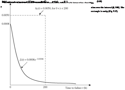
Solution Referring to Example 6.7, uniform distribution U(0, 200) has a height of 0.005 (see Fig. 6.8). The antithetic-variate method along with the sample-mean Monte Carlo algorithm for evaluating the pump failure probability can be outlined as follows:

1. Generate n pairs standard uniform random variates (ui,1 — Ui) from U(0, 1).

2. Let tn = 200 Ui and t^i = 200(1 — Ui). Compute ft(tn) and ft(t2i).

3. Estimate the pump failure probability, according to Eq. (6.79), as

Pf, a = 200 £[ ft (hi) + ft (t2i)]

i=1

Using this algorithm, the estimated pump failure probability is pf = 0.14785. Comparing with the exact failure probability pf = 0.147856, the estimated failure probability by the antithetic-variates algorithm with n = 1000 and the simple uniform distribution is accurate within 0.00406 percent. The standard deviation s associated with the 2n random samples is 0.00669. According to Eq. (6.74), the standard error associated with pif a can be computed as s/V2n = 0.00015. The skewness coefficient from the 2n random samples is 0.077, which is close to zero. Hence, by the normal­ity approximation, the 95 percent confidence interval containing the exact failure probability pf is (0.14756, 0.14814).

Comparing the solutions with those of Examples 6.6, 6.7, and 6.9, it is observed that the antithetic-variate algorithm is very accurate in estimating the probability.

The importance sampling technique concentrates the distribution of sampling points in the part of the domain that is most “important” for the task rather than spreading them out evenly (Marshall, 1956). Refer to the problem of evaluating an integral in Eq. (6.49) by the sample-mean method. The importance sampling technique attempts to generate M sampling points to reduce the variance of G given by Eq. (6.61).

Rubinstein (1981) showed that the PDF fx(x) that minimizes Eq. (6.61) can be obtained as

|g (x)| / |g (x)| dx
fx(x)	(6.72)
Although Eq. (6.72) indicates that the weighing function fx(x) is a function of / |g (x)| dx, which is practically equivalent to the integral sought, however, it is not completely useless. Equation (6.72) implies that if is fx(x) is chosen to have a similar shape as |g (x)|, considerable reduction in variance of the simulation results can be achieved. However, in practical implementations of this technique, consideration must be given to the tradeoffbetween the desired error reduction and the difficulties of sampling from fx (x), especially when |g (x)| is not well behaved.
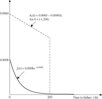
Example 6.9 Repeat Example 6.6 using the importance sampling technique with n = 2000. The PDF selected is a trapezoidal distribution with a PDF defined as ht(t) = 0.006 — b x t for 0 < t < 200
where b is the slope of the dashed line shown in Fig. 6.12. Compare the efficiency of the technique under this distribution with that in Examples 6.6 and 6.7.
Solution Using the importance sampling method with the trapezoidal PDF indicated earlier, evaluation of the pump failure probability can be expressed as
(i)

From condition (i), the coefficient b can be obtained easily as b = 0.00001. Substituting b = 0.00001 into ht(t), one can verify that condition (ii) is also satisfied. Therefore, ht(t) = 0.006 — 0.00001 x t is a legitimate PDF in 0 < t < 200. To generate random variates from ht(t), the CDF-inverse method can be used because the CDF of ht(t) can be obtained easily as

Ht(T) = U = (0.006 — 0.00001t) dt = 0.006T — ^°-002001) T 2

Solving for T in terms of U, one obtains

in which a = 0.006 and b = 0.00001. Based on the boundary conditions of a CDF, that is, Ht(t = 0) = 0 and Ht(t = 200) = 1, the only valid expression for T from ht(t) is

T 2a — V 4a2 — 8bU

= 2b

Hence the preceding equation can be used to generate random variates from ht(t). The algorithm for this example can be outlined as follows:

1. Generate n standard uniform random variates ui from U(0, 1).

2. Compute ti according to Eq. (6.73), yielding n random variates from ht(t) = 0.006 —

0. 00001t, 0 < t < 200.

3. Estimate the pump failure probability as

4. To assess the error associated with the estimated pump failure probability by the preceding equation, compute the following quantity:

(6.74)

2

pZ

Using this algorithm, the estimated pump failure probability is pf = 0.14767, whereas the exact failure probability is 0.147856. The associated standard error can be computed as

sp f = 0.00023

Assuming normality for the estimated pump failure probability, the 95 percent confi­dence interval containing the exact risk pf is

pf ± 1.96spf = (0.14722,0.14813)

Comparing the solutions with those of Examples 6.6 and 6.7, it is observed that with the same n = 2000, the importance sampling method has a 0.126 percent error. The magnitude of error and the accuracy level are somewhat worse than the sample- mean procedure but are still far better than the hit-and-miss algorithm. The accuracy of the importance sampling technique depends on how ht(t) is specified. As can be observed from Problem 6.29, use of the exponential function for ft(t) improves the accuracy tremendously.

Since Monte Carlo simulation is a sampling procedure, results obtained from the procedure inevitably involve sampling errors, which decrease as the sam­ple size increases. Increasing the sample size to achieve a higher precision generally means an increase in computer time for generating random vari­ates and data processing. Variance-reduction techniques aim at obtaining high accuracy for the Monte Carlo simulation results without having to substan­tially increase the sample size. Hence variance-reduction techniques enhance the statistical efficiency of the Monte Carlo simulation. When applied properly, variance-reduction techniques sometimes can make the difference between an impossible, expensive, simulation study and a feasible, useful one.

Variance-reduction techniques attempt to reduce the error associated with the Monte Carlo simulation results by using known information about the prob­lem at hand. Naturally, such an objective cannot be attained if the analyst is completely ignorant about the problem. On the other extreme, the error is zero if the analyst has complete knowledge about the problem. Rubinstein (1981) stated that “variance reduction cannot be obtained from nothing; it is merely a way of not wasting information.” Therefore, for a problem that is not known at the initial stage of the study, pilot simulations can be performed for the purpose of gaining useful insight into the problem. The insight, then, can be incorporated later into the variance-reduction techniques for a more efficient

simulation study. Therefore, most of the variance-reduction techniques require additional effort on the part of analysts.

Referring to Monte Carlo integration, different algorithms yield different esti­mators for the integral. A relevant issue is which algorithm is more efficient. The efficiency issue can be examined from the statistical properties of the esti­mator from a given algorithm and its computational aspects. Rubinstein (1981) showed a practical measure of the efficiency of an algorithm by t x Var(©), with t being the computer time required to compute ©, which estimates ©. Algorithm 1 is more efficient than algorithm 2 if

If the computational times for the two algorithms are approximately equal, comparison of efficiency can be made by examining the relative magnitude of the variances. When the true variances are not known, which is generally the case, sample variances can be used. Without considering the computational time, it can be shown that the sample-mean algorithm using X ~ U(a, b) is more efficient than the hit-and-miss algorithm (see Problem 6.25).

Consider the reliability computation involving a multidimensional integral as Eq. (6.48). Without losing generality, the following discussions assume that the stochastic variables in the original X-space have been transformed to the independent standard normal Z’-space (see Sec. 2.7.2). Consequently, the orig­inal performance function W(X) can be expressed as W(Z’). In terms of Z Eq. (6.48) can be written as

	(6.64)

in which ф (z 0 is the K-dimensional joint PDF of independent standard normal random variables Z’.

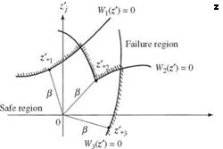
Analytical solutions to Eq. (6.64) exist for only a few special cases. For most problems, Eq. (6.64) is solved by approximation methods, such as the first – and second-order reliability methods described in Secs. 4.4 through 4.6. Note that the advanced first-order second-moment methods and the second-order reliability methods require identification of the design point (or points) on the failure surface defined by W (z’) = 0. For problems involving multiple design points or a single design point with several points having almost the same distance, they can be cast into the system reliability framework described in Chap. 5. Nevertheless, the process of identifying designing points involves non­linear optimization, by which the search for all design points is a difficult task for problems having a complex failure surface defined by several performance functions (Fig. 6.9).

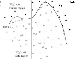
By the simple Monte Carlo simulation, n sets of random vector z’ are pro­duced to compute the corresponding values of the performance function W (z 0. The unbiased estimator of the reliability of a system is the ratio between the number of outcomes in the safe region [with W(z’) > 0] and the total number of random sets generated n (Fig. 6.10). The Monte Carlo simulation applying simple random sampling, in general, is not efficient, especially when the failure probability is very small. Directional simulation is a simple procedure based on the idea of conditional probability to improve the efficiency of the Monte Carlo

solution in Eq. (6.64). The procedure can be applied jointly with the variance reduction techniques described in Sec. 6.7 to further improve the computational efficiency and numerical accuracy of the Monte Carlo simulation of reliability problems.

In the K-dimensional Z’-space, any Gaussian random vector Z’ can be ex­pressed as

Z’ = RE (6.65)

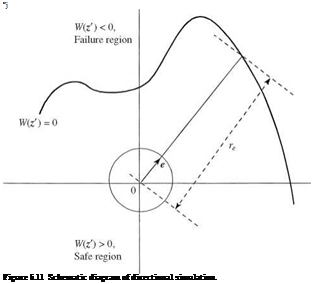
where R > 0 is chi-square random variable with K degrees of freedom, and E = (E1, E2,…, EK), an independent random unit vector of length one, that is, E | = 1. The random unit vector E is uniformly distributed on the K-dimensional unit hypersphere RK. Along a specific direction E = e, the conditional reliabil­ity pse is

Ps |e = P [W(г’) > 0] = P [W(Re) > 0] = P [R < ^] = Fg (r?) (6.66)

in which z ‘e = Re is a vector having a random length R along the direction defined by the vector e, re is the distance from the origin to the failure sur­face along the vector e satisfying W(ree) = 0, and Fx|( ) is the x[16] CDF with K degrees of freedom. The geometric definitions of the terms in Eq. (6.66) are shown in Fig. 6.11. Note that the distance re has to be found by a suitable method. For a complicated performance function, numerical root-finding tech­niques have to be used. If the safe region is nonclosed, the root is for some e. As can be seen, if the failure surface is a hypersphere, the reliability can be found by a single trial in the directional simulation.

From ps |e, the reliability can be obtained using the total probability theorem (Sec. 2.2.4) as

ps = (ps|e) fe (e) de (6.67)

ee Rk

where f e(e) is the density function of random unit vector E on the unit hyper­sphere, which is a constant. The realization of the random unit vector can be ob­tained easily as e = z’/|z’|, with z’ being a randomly generated vector contain­ing K independent standard normal variates. As can be seen from Eq. (6.67), the reliability of the conditional simulation is the expectation of the conditional reliability, that is, Ee(ps|e). Therefore, similar to the sample-mean Monte Carlo integration, the reliability can be estimated as

where n is the total number of repetitions in the simulation, ps i = ps |ei, ei is the unit vector randomly generated in the ith repetition, and ri is the distance from the origin in the Z – space to the failure surface from solving W (riei) = 0. The directional simulation algorithm can be implemented as follows: [17] 2

3. Determine the distance re from the origin to the failure surface by solving W (ree) = 0.

4. Compute the conditional reliability ps, i = Fx|(re).

5. Repeat steps 2 through 4 n times, obtaining {ps1, ps,2,, ps, n}.

6. Compute the reliability by Eq. (6.68).

The standard error associated with the reliability estimated by Eq. (6.108) is

1 n

Var(ps) = ——————– — У2 (Ps, i – ps)2 (6.69)

n(n – 1)

i = 1

If the number of samples n is large, the estimated reliability ps can be treated as a normal random variable (according to the central limit theorem), with the variance given by Eq. (6.69). Then the 95 percent confidence interval for the true reliability ps can be obtained as

Ps ± 1.96[Var(ps)]a5 (6.70)

Since the directional simulation yields the exact solution for the reliability integral when the failure surface is a hypersphere in the Z’-space, Bjerager (1988) indicated that the procedure will be particularly efficient for problems where the failure surface is “almost spherical.” Furthermore, owing to the an­alytical evaluation of the conditional reliability in Eq. (6.66), the directional simulation will yield a smaller variance on the reliability estimator for a given sample size n than that of the simple random sampling procedure. Bjerager (1988) demonstrated the directional simulation through several examples and showed that the coefficient of variation of estimated reliability ps for a given sample size depends on the shape of the failure surface and the value of the un­known reliability. For nonspherical failure surfaces, the coefficient of variation increases as the dimensionality of the problem K increases.

Example 6.8 Refer to the slope stability problem in Example 6.4. Use the directional simulation to estimate the probability that the excavation can be performed safely within 40 days.

Solution Referring to Eq. (6.29), the problem is to find the probability that the random drawdown recess time will be less than or equal to 40 days, that is,

in which d = 50 m, ho = 30 m, and S and Kh are the random storage coefficient and conductivity, having a bivariate normal distribution. The means and standard deviations of S and Kh are, respectively, /xs = 0.05, iikh = 0.1 m/day, as = 0.005,

akh = 0.01 m/day, and their correlation coefficient is Pkh, s = 0-5- The corresponding performance function can be expressed as

W(Kh, S) = S – cKh

where c = 0.43686.

By the directional simulation outlined earlier, the stochastic variables involved are transformed to the independent standard normal space. For this example, the random conductivity Kh and storage coefficient S can be written in terms of the independent normal random variables Z1 and Z2 by spectral decomposition as

Kh = 0.1 + 0.005 (Z1 + V3 Z2)

S = 0.05 – 0.0025 (Z1 – V3Z2)

For each randomly generated direction vector, defined by z’ = (z^, z2), the compo­nents of the corresponding unit vector e = (e1, 62)* can be computed by normalizing the vector z’. Therefore, along the directional vector z’, the values of the conductivity and storage coefficient can be expressed in terms of the unit vector e and the length of the vector re from the origin to the failure surface in the independent standard normal space as

Kh = 0.1 + 0.005re (б1 + л/3б2)

S = 0.05 – 0.0025r6 (є 1 – V3e2)

Substituting the preceding expression for Kh and S into the performance function, the failure surface, defined by W(kh, s) = W(r6e) = 0, can be explicitly written as

s – kh = [0.05 – 0.0025r6 (є1 – л/3є^] – c [0.1 + 0.005r6(є1 + л/3є^| = 0

Because the performance function in this example is linear, the distance гє can be solved easily as

0. 006314432

0. 0046842784є1 – 0.0005468459є2

For a more complex, nonlinear performance function, proper numerical root-finding procedures must be applied. Furthermore, a feasible direction e should be the one that yields a positive-valued re.

The algorithm P (T < 40) by the directional simulation for this example can be summarized as follows:

1. Generate two independent standard normal variates and z2.

2. Compute the elements of the corresponding unit vector e.

3. Compute the value of distance variable re. If re < 0, reject the current infeasible direction and go back to step 1 for a new direction. Otherwise, go to step 4.

4. Compute P(T < 40|e) = 1 – F 2(гє), and store the results.

X2

5. Repeat steps 1 throught 4 a large number of times n.

6. Compute the average conditional probability as the estimate for P (T < 40) according to Eq. (6.68). Also calculate the associated standard error of the esti­mate by Eq. (6.69) and the confidence interval.

Based on n = 400 repetitions, the directional simulation yields an estimation of P(T < 40) ^ 0.026141 associated with a standard error of0.001283. By the normality assumption, the 95 percent confidence interval is (0.023627, 0.028655).

The sample-mean Monte Carlo integration is based on the idea that the com­putation of the integral by Eq. (6.49) alternatively can be carried out by

in which fx(x) > 0 is a PDF defined over a < x < b. The transformed in­tegral given by Eq. (6.49) is equivalent to the computation of expectation of g(X)/fx (X), namely,

with X being a random variable having a PDF fx(x) defined over a < x < b. The estimation of E [g(X)/fx(X)] by the sample-mean Monte Carlo integration method is

G _ 1 g(xi)

n fx (xi)

in which xi is the random variate generated according to fx(x), and n is the number of random variates produced. The sample estimator given by Eq. (6.60) has a variance

The sample-mean Monte Carlo integration algorithm can be implemented as follows:

For simplicity, consider that X ~ U(a, b) has a PDF

1

b – a

The sample-mean algorithm, then, can be outlined as the following:

1. Generate n standard uniform random variates ui from U(0, 1).

2. Let ti = 200ui, which is a uniform random variate from U(0, 200), and compute ft (ti).

3.

Estimate the pump failure probability as

4.

To assess the error associated with the estimated pump failure probability by the preceding equation, compute the following quantity:

where (•) is the operator for the mean of the quantity inside.

Using this algorithm for 2000 simulations, the estimated pump failure probability is pf = 0.14797. Comparing with the exact failure probability, pf = 0.147856, the estimated failure probability by the sample-mean method, with n = 2000 and the simple uniform distribution chosen, has an error of0.0771 percent relative to the exact solution.

The associated standard error can be computed according to Eq. (6.63) as

spf = ^(pf ) – (pf )2 = 0.00015

Assuming normality for the estimated pump failure probability, the 95 percent confi­dence interval containing the exact failure probability pf is

pf + 1.96 spf = (0.14767,0.14826)

Comparing the solutions with those of Example 6.6, it is observed that for the same number ofsamples n, the sample-mean algorithm yields a significantly more accurate estimation than the hit-and-miss algorithm. Furthermore, the precision, represented by the standard error, associated with the estimated failure probability by the sample – mean method, is smaller than that of the hit-and-miss algorithm. Consequently, the confidence interval with the same level of significance will be tighter.

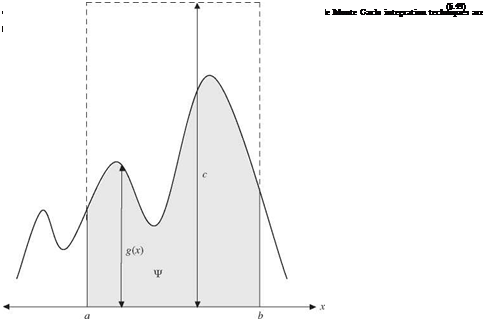
Referring to Fig. 6.6, a rectangular region Ш = {(x, y)a < x < b, 0 < y < c} is superimposed to enclose the area Ф = {(x, y)a < x < b, 0 < y = g(x) < c} represented by Eq. (6.49). By the hit-and-miss method, the rectangular region Ш containing the area under g(x), that is, Ф, is hung on the wall, and one is to throw n darts on it. Assume that the darts fly in a random fashion and that all n darts hit within the rectangular region. The area under g(x), then, can be estimated as the proportion of n darts hitting the target multiplied by the known area of rectangular region Ш, that is,

G = A(6.50)

where G is the estimate of the true area G under g(x), A = c(b – a) is the area of the rectangular region, and nh is the number of darts hitting the target out of a total of n trials.

The hit-and-miss method can be implemented numerically on a computer. The two coordinates (Xi, Yi) on the rectangular region Ш, which represents the location where the ith dart lands, are treated as two independent random variables that can be generated from two uniform distributions. That is, Xi is generated from U(a, b) and Yi from U(0, c). When Yi < g(Xi), the dart hits its target; otherwise, the dart misses the target. A simple hit-and-miss algorithm is given as follows:

1. Generate 2n uniform random variates from U(0, 1). Form them arbitrarily into n pairs, that is, (u1, u[), (u2, u’2),…, (un, u’n).

2. Compute xi = a + (b – a)ui and g(xi), for i = 1,2,…, n.

3. Count the number of cases nh that g(xt) > cu.

4. Estimate the integral G by Eq. (6.50).

Note that G is an estimator of the integral G; it is therefore also a random variable. It can be shown that G is unbiased, namely,

E(G) = A x = Ap = A (A = G (6.51)

where nh/n, the proportion of n darts hitting the target, is an unbiased estimator of the true probability of hits, and p simply is the ratio of the area under g(x) to the area of the rectangular region. Furthermore, the standard error associated with the estimator G is

As can be seen, the precision associated with G, represented by its inverse of standard deviation, using the hit-and-miss Monte Carlo integration method increases with n1/2.

A practical question is how many trials have to be carried out so that the estimated G satisfies a specified accuracy requirement. In other words, one would like to determine a minimum number of trials n such that the following relationship holds:

P(|G – G<e) > a (6.53)

in which є is the specified maximum error between G and G, and a is the mini­mum probability that G would be within є around the exact solution. Applying the Chebyshev inequality, the minimum number of trials required to achieve Eq. (6.53) can be determined as (Rubinstein, 1981)

(1 – p)p[c(b – a)]2 (1 – p)pA2

n >———— / 2——— = n * 2 (6.54)

(1 – а)є2 (1 – а)є2

Note that the required number of trials n increases as the specified error level є decreases and as the confidence level a increases. In addition, for the specified є and a, Eq. (6.54) indicates that the required number of trials n can be reduced by letting p approach 1. This implies that selecting an enclosed region Ш as close to Ф as possible would reduce the required number of trials. However, consideration must be given to the ease of generating random variates for U’ in the algorithm.

When the number of trials n is sufficiently large, the random variable T,

G — G

T = ^^ (6.55)

sG

approximately, has the standard normal distribution, that is, T ~ N(0, 1), with sG being the sample estimator of aG, that is,

Hence the (1 – 2a)-percent (a < 0.5) confidence interval for G then can be ob­tained as

G ± sgza

with za = Ф 1(1 – a).

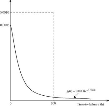
Example 6.6 Suppose that the time to failure of a pump in a water distribution system follows an exponential distribution with the parameter в = 0.0008/h (i. e., 7 failures per year). The PDF of the time to failure of the pump can be expressed as

ft(t) = 0.0008e-0 0008t for t > 0

Determine the failure probability of the pump within its first 200 hours of operation by the hit-and-miss algorithm with n = 2000. Also compute the standard deviation associated with the estimated failure probability and derive the 95 percent confidence interval containing the exact failure probability.

Solution The probability that the pump would fail within 200 hours can be computed as

r-200 ,■ 200

ft (t) dt = 0.0008e—00008t dt

00 which is the area under the PDF between 0 and 200 hours (Fig. 6.7). Using the hit – and-miss Monte Carlo method, a rectangular area with a height of 0.0010 over the interval [0, 200] is imposed to contain the area representing the pump failure proba­bility.

The area of the rectangle can be easily determined as A = 0.001(200) = 0.2. The hit-and-miss algorithm then can be outlined in the following steps:

1. Initialize i = 0 and щ = 0.

2. Let i = i + 1, and generate a pair of standard uniform random variates (ui, ui) from U(0, 1).

3. Let ti = 200ui, and compute ft(ti) = 0.0008e—00008ti, y = 0.001ui.

4. If ft(ti) > y, nh = nh + 1. If i = 2000, go to step 5; otherwise, go to step 1.

5. Estimate the pump failure probability as pf = A(nh/n) = 0.2(nh/n).

Using the preceding algorithm, 2000 simulations were made, and the estimated pump failure probability is pif = 0.2(nh/n) = 0.2(1500/2000) = 0.15. Comparing with the exact failure probability pf = 1 — exp(-0.16) = 0.147856, the estimated

failure probability by the hit-and-miss method, with n = 2000 and the rectangular area chosen, has a 1.45 percent error relative to the exact solution.

The associated standard error can be computed according to Eq. (6.56) as

Assuming normality for the estimated pump failure probability, the 95 percent confi­dence interval containing the exact failure probability pf is

pf ± Z0.975SPf = (0.1462,0.1538)

where zq.975 = 1.96.

In reliability analysis, computations of system and/or component reliability and other related quantities, such as mean time to failure, essentially involve inte­gration operations. A simple example is the time-to-failure analysis in which the reliability of a system within a time interval (0, t) is obtained from

where ft (t) is the failure density function. A more complex example of the reli­ability computation is by load-resistance interference in that the reliability is

Ps = P[R(Xr) > L(Xl)] = P [W(Xr, Xl) > 0] = P [W(X) > 0]

= f fx (x) dx (6.48)

JW (x)>0

where R(XR) and L(XL) are, respectively, resistance and load functions, which are dependent on some basic stochastic variables XR = (X1, X2,…, Xm) and XL = (Xm+1,Xm+2,…,XK), and W(X) is the performance function. As can be seen, computation of reliability by Eq. (6.48) involves K-dimensional integrations.

For cases of integration in one or two dimensions, such as Eq. (6.47), where the integrands are well behaved (e. g., no discontinuity), conventional numer­ical integration methods, such as the trapezoidal approximation or Simpson’s rule (see Appendix 4A), are efficient and accurate. For example, using Simp­son’s rule, the error in a one-dimensional integration is O(n-4), with n being the number of discretizations, and the error in a two-dimensional integration is O(n-2). Gould and Tobochnik (1988) show that, in general, if the error for the one-dimensional integration is O(n-a), the error with a K-dimensional in­tegration would be O(n~a/K). As can be seen, the accuracy of conventional nu­merical integration schemes decreases rapidly as the dimension of integration increases. For multiple integrals, such as Eq. (6.48), the Monte Carlo method becomes a more suitable numerical technique for integration.

To illustrate the basic idea of the Monte Carlo integration, consider a simple one-dimensional integration

Procedures described in Sec. 6.5.2 are for generating multivariate normal (Gaussian) random variables without imposing constraints or restriction on the values of variates. The procedures under this category are also called uncon­ditional (or nonconditional) simulation (Borgman and Faucette, 1993; Chiles and Delfiner, 1999). In hydrosystems modeling, random variables often exist for which, in addition to their statistical correlation, they are physically related in certain functional forms. In particular, this section describes the procedures for generating multivariate Gaussian random variates that must satisfy pre­scribed linear relationships. An example is the use of unit hydrograph model for estimating design runoff based on a design rainfall excess hyetograph. The unit hydrograph is applied as follows:

Pu= q (6.38)

where P is an n x J Toeplitz matrix defining the design effective rainfall hyeto­graph, u is a J x 1 column vector of unit hydrograph ordinates, and q is the n x 1 column vector of direct runoff hydrograph ordinates. In the process of deriving a unit hydrograph for a watershed, there exist various uncertainties rendering u uncertain. Hence the design runoff hydrograph q obtained from Eq. (6.38) is subject to uncertainty. Therefore, to generate a plausible direct runoff hydrograph for a design rainfall excess hyetograph, one could generate unit hydrographs that must consider the following physical constraint:

J

Y^Uj = c (6.39)

j=1

in which c is a constant to ensure that the volume of unit the hydrograph is one unit of effective rainfall.

The linearly constrained Monte Carlo simulation can be conducted by using the acceptance-rejection method first proposed by von Neumann (1951). The AR method generally requires a large number of simulations to satisfy

the constraint and, therefore, is not computationally efficient. Borgman and Faucettee (1993) developed a practical method to convert a Gaussian linearly constrained simulation into a Gaussian conditional simulation that can be im­plemented straightforwardly. The following discussions will concentrate on the method of Borgman and Faucette (1993).

Conditional simulation (CS) was developed in the field of geostatistics for modeling spatial uncertainty to generate a plausible random field that honors the actual observational values at the sample points (Chiles and Delfiner, 1999). In other words, conditional simulation yields special subsets of realizations from an unconditional simulation in that the generated random variates match with the observations at the sample points. For the multivariate normal case, the Gaussian conditional simulation is to simulate a normal random vector X2 con­ditional on the normal random vector X1 = x1*. To implement the conditional simulation, define a new random vector X encompassing of Xi and X2 as

generated conditioned on y1 = b. Hence, using the spectral decomposition de­scribed in Sec. 6.5.2.2, random vector X subject to linear constraints Eq. (6.42) can be obtained in the following two steps:

1. Calculate (m + K)-dimensional multivariate normal random vector y by un­conditional simulation as

У = (yO = VyA-°y5 Z + Ъ (6.45)

where y1 is an m x 1 column vector, y2 is a K x 1 column vector; Vy is an (m + K) x (m + K) eigenvector matrix of Cy, and Лу is a diagonal matrix of eigenvalues of Cy, and Z’ is an (m + K) column vector of independent standard normal variates.

2. Calculate the linearly constrained K-dimensional vector of random variates x, according to Eq. (6.41), as

x = y2* = y2 + C y,12C-,n(b – y1) (6.46)

This constrained multivariate normal simulation has been applied, by con­sidering the uncertainties in the unit hydrograph and geomorphologic instan­taneous unit hydrograph, to reliability analysis of hydrosystems engineering infrastructures (Zhao et al., 1997a, 1997b; Wang and Tung, 2005).

In many practical hydrosystems engineering problems, random variables often are statistically and physically dependent. Furthermore, distribution types for the random variables involved can be a mixture of different distributions, of which the corresponding joint PDF or CDF is difficult to establish. As a practical alternative, to replicate such systems properly, the Monte Carlo simulation should be able to preserve the correlation relationships among the stochastic variables and their marginal distributions.

In a multivariate setting, the joint PDF represents the complete information describing the probabilistic structures of the random variables involved. When the joint PDF or CDF is known, the marginal distribution and conditional dis­tributions can be derived, from which the generation of multivariate random variates can be made straightforwardly in the framework of Rosenblatt (1952). However, in most practical engineering problems involving multivariate ran­dom variables, the derivation of the joint CDF generally is difficult, and the availability of such information is rare. The level of difficulty, in both theory and practice, increases with the number of random variables and perhaps even more so by the type of corresponding distributions. Therefore, more often than not, one has to be content with preserving incomplete information represented by the marginal distribution of each individual random variable and the corre­lation structure. In doing so, the difficulty of requiring a complete joint PDF in the multivariate Monte Carlo simulation is circumvented.

To generate correlated random variables with a mixture of marginal distribu­tions, a methodology adopting a bivariate distribution model was first suggested by Li and Hammond (1975). The practicality of the approach was advanced by Der Kiureghian and Liu (1985), who, based on the Nataf bivariate distribution model (Nataf, 1962), developed a set of semiempirical formulas so that the nec­essary calculations to preserve the original correlation structure in the normal transformed space are reduced (see Table 4.5). Chang et al. (1994) used this set of formulas, which transforms the correlation coefficient of a pair of nonnor­mal random variables to its equivalent correlation coefficient in the bivariate standard normal space, for multivariate simulation. Other practical alterna­tives, such as the polynomial normal transformation (Vale and Maurelli, 1983; Chen and Tung, 2003), can serve the same purpose. Through a proper normal transformation, the multivariate Monte Carlo simulation can be performed in a correlated standard normal space in which efficient algorithms, such as those described in Sec. 6.5.2, can be applied.

The Monte Carlo simulation that preserves marginal PDFs and correlation structure of the involved random variables consists of following two basic steps:

Step 1. Transformation to a standard normal space. Through proper normal transformation, the operational domain is transformed to a standard normal space in which the transformed random variables are treated as if they were multivariate standard normal with the correlation matrix Rz. As a result, multivariate normal random variates can be generated by the techniques described in Sec. 6.5.2.

Step 2. Inverse transformation. Once the standardized multivariate normal random variates are generated, then one can do the inverse transformation

Xk = ^[Ф( Zk)] for k = 1,2,…, K (6.37)

to compute the values of multivariate random variates in the original space.