The sample-mean method

The sample-mean Monte Carlo integration is based on the idea that the com­putation of the integral by Eq. (6.49) alternatively can be carried out by

in which fx(x) > 0 is a PDF defined over a < x < b. The transformed in­tegral given by Eq. (6.49) is equivalent to the computation of expectation of g(X)/fx (X), namely,

with X being a random variable having a PDF fx(x) defined over a < x < b. The estimation of E [g(X)/fx(X)] by the sample-mean Monte Carlo integration method is

G _ 1 g(xi)

n fx (xi)

fx(x) dx – G[13] [14] [15]

in which xi is the random variate generated according to fx(x), and n is the number of random variates produced. The sample estimator given by Eq. (6.60) has a variance

The sample-mean Monte Carlo integration algorithm can be implemented as follows:

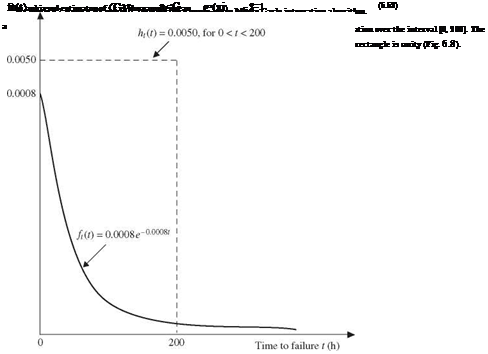
For simplicity, consider that X ~ U(a, b) has a PDF

1

b – a

The sample-mean algorithm, then, can be outlined as the following:

1. Generate n standard uniform random variates ui from U(0, 1).

2. Let ti = 200ui, which is a uniform random variate from U(0, 200), and compute ft (ti).

3.

Estimate the pump failure probability as

4.

To assess the error associated with the estimated pump failure probability by the preceding equation, compute the following quantity:

where (•) is the operator for the mean of the quantity inside.

Using this algorithm for 2000 simulations, the estimated pump failure probability is pf = 0.14797. Comparing with the exact failure probability, pf = 0.147856, the estimated failure probability by the sample-mean method, with n = 2000 and the simple uniform distribution chosen, has an error of0.0771 percent relative to the exact solution.

The associated standard error can be computed according to Eq. (6.63) as

spf = ^(pf ) – (pf )2 = 0.00015

Assuming normality for the estimated pump failure probability, the 95 percent confi­dence interval containing the exact failure probability pf is

pf + 1.96 spf = (0.14767,0.14826)

Comparing the solutions with those of Example 6.6, it is observed that for the same number ofsamples n, the sample-mean algorithm yields a significantly more accurate estimation than the hit-and-miss algorithm. Furthermore, the precision, represented by the standard error, associated with the estimated failure probability by the sample – mean method, is smaller than that of the hit-and-miss algorithm. Consequently, the confidence interval with the same level of significance will be tighter.