Directional Monte Carlo simulation algorithm
Consider the reliability computation involving a multidimensional integral as Eq. (6.48). Without losing generality, the following discussions assume that the stochastic variables in the original X-space have been transformed to the independent standard normal Z’-space (see Sec. 2.7.2). Consequently, the original performance function W(X) can be expressed as W(Z’). In terms of Z Eq. (6.48) can be written as
|
||
in which ф (z 0 is the K-dimensional joint PDF of independent standard normal random variables Z’.
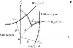
Analytical solutions to Eq. (6.64) exist for only a few special cases. For most problems, Eq. (6.64) is solved by approximation methods, such as the first – and second-order reliability methods described in Secs. 4.4 through 4.6. Note that the advanced first-order second-moment methods and the second-order reliability methods require identification of the design point (or points) on the failure surface defined by W (z’) = 0. For problems involving multiple design points or a single design point with several points having almost the same distance, they can be cast into the system reliability framework described in Chap. 5. Nevertheless, the process of identifying designing points involves nonlinear optimization, by which the search for all design points is a difficult task for problems having a complex failure surface defined by several performance functions (Fig. 6.9).
 |
|
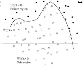
By the simple Monte Carlo simulation, n sets of random vector z’ are produced to compute the corresponding values of the performance function W (z 0. The unbiased estimator of the reliability of a system is the ratio between the number of outcomes in the safe region [with W(z’) > 0] and the total number of random sets generated n (Fig. 6.10). The Monte Carlo simulation applying simple random sampling, in general, is not efficient, especially when the failure probability is very small. Directional simulation is a simple procedure based on the idea of conditional probability to improve the efficiency of the Monte Carlo

solution in Eq. (6.64). The procedure can be applied jointly with the variance reduction techniques described in Sec. 6.7 to further improve the computational efficiency and numerical accuracy of the Monte Carlo simulation of reliability problems.
In the K-dimensional Z’-space, any Gaussian random vector Z’ can be expressed as
Z’ = RE (6.65)
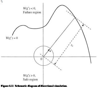
where R > 0 is chi-square random variable with K degrees of freedom, and E = (E1, E2,…, EK), an independent random unit vector of length one, that is, E | = 1. The random unit vector E is uniformly distributed on the K-dimensional unit hypersphere RK. Along a specific direction E = e, the conditional reliability pse is
Ps |e = P [W(г’) > 0] = P [W(Re) > 0] = P [R < ^] = Fg (r?) (6.66)
in which z ‘e = Re is a vector having a random length R along the direction defined by the vector e, re is the distance from the origin to the failure surface along the vector e satisfying W(ree) = 0, and Fx|( ) is the x[16] CDF with K degrees of freedom. The geometric definitions of the terms in Eq. (6.66) are shown in Fig. 6.11. Note that the distance re has to be found by a suitable method. For a complicated performance function, numerical root-finding techniques have to be used. If the safe region is nonclosed, the root is for some e. As can be seen, if the failure surface is a hypersphere, the reliability can be found by a single trial in the directional simulation.
 |
From ps |e, the reliability can be obtained using the total probability theorem (Sec. 2.2.4) as
ps = (ps|e) fe (e) de (6.67)
ee Rk
where f e(e) is the density function of random unit vector E on the unit hypersphere, which is a constant. The realization of the random unit vector can be obtained easily as e = z’/|z’|, with z’ being a randomly generated vector containing K independent standard normal variates. As can be seen from Eq. (6.67), the reliability of the conditional simulation is the expectation of the conditional reliability, that is, Ee(ps|e). Therefore, similar to the sample-mean Monte Carlo integration, the reliability can be estimated as
where n is the total number of repetitions in the simulation, ps i = ps |ei, ei is the unit vector randomly generated in the ith repetition, and ri is the distance from the origin in the Z – space to the failure surface from solving W (riei) = 0. The directional simulation algorithm can be implemented as follows: [17] 2
3. Determine the distance re from the origin to the failure surface by solving W (ree) = 0.
4. Compute the conditional reliability ps, i = Fx|(re).
5. Repeat steps 2 through 4 n times, obtaining {ps1, ps,2,, ps, n}.
6. Compute the reliability by Eq. (6.68).
The standard error associated with the reliability estimated by Eq. (6.108) is
1 n
Var(ps) = ——————– — У2 (Ps, i – ps)2 (6.69)
n(n – 1)
i = 1
If the number of samples n is large, the estimated reliability ps can be treated as a normal random variable (according to the central limit theorem), with the variance given by Eq. (6.69). Then the 95 percent confidence interval for the true reliability ps can be obtained as
Ps ± 1.96[Var(ps)]a5 (6.70)
Since the directional simulation yields the exact solution for the reliability integral when the failure surface is a hypersphere in the Z’-space, Bjerager (1988) indicated that the procedure will be particularly efficient for problems where the failure surface is “almost spherical.” Furthermore, owing to the analytical evaluation of the conditional reliability in Eq. (6.66), the directional simulation will yield a smaller variance on the reliability estimator for a given sample size n than that of the simple random sampling procedure. Bjerager (1988) demonstrated the directional simulation through several examples and showed that the coefficient of variation of estimated reliability ps for a given sample size depends on the shape of the failure surface and the value of the unknown reliability. For nonspherical failure surfaces, the coefficient of variation increases as the dimensionality of the problem K increases.
Example 6.8 Refer to the slope stability problem in Example 6.4. Use the directional simulation to estimate the probability that the excavation can be performed safely within 40 days.
Solution Referring to Eq. (6.29), the problem is to find the probability that the random drawdown recess time will be less than or equal to 40 days, that is,
in which d = 50 m, ho = 30 m, and S and Kh are the random storage coefficient and conductivity, having a bivariate normal distribution. The means and standard deviations of S and Kh are, respectively, /xs = 0.05, iikh = 0.1 m/day, as = 0.005,
akh = 0.01 m/day, and their correlation coefficient is Pkh, s = 0-5- The corresponding performance function can be expressed as
W(Kh, S) = S – cKh
where c = 0.43686.
By the directional simulation outlined earlier, the stochastic variables involved are transformed to the independent standard normal space. For this example, the random conductivity Kh and storage coefficient S can be written in terms of the independent normal random variables Z1 and Z2 by spectral decomposition as
Kh = 0.1 + 0.005 (Z1 + V3 Z2)
S = 0.05 – 0.0025 (Z1 – V3Z2)
For each randomly generated direction vector, defined by z’ = (z^, z2), the components of the corresponding unit vector e = (e1, 62)* can be computed by normalizing the vector z’. Therefore, along the directional vector z’, the values of the conductivity and storage coefficient can be expressed in terms of the unit vector e and the length of the vector re from the origin to the failure surface in the independent standard normal space as
Kh = 0.1 + 0.005re (б1 + л/3б2)
S = 0.05 – 0.0025r6 (є 1 – V3e2)
Substituting the preceding expression for Kh and S into the performance function, the failure surface, defined by W(kh, s) = W(r6e) = 0, can be explicitly written as
s – kh = [0.05 – 0.0025r6 (є1 – л/3є^] – c [0.1 + 0.005r6(є1 + л/3є^| = 0
Because the performance function in this example is linear, the distance гє can be solved easily as
0. 006314432
0. ![]() 0046842784є1 – 0.0005468459є2
0046842784є1 – 0.0005468459є2
For a more complex, nonlinear performance function, proper numerical root-finding procedures must be applied. Furthermore, a feasible direction e should be the one that yields a positive-valued re.
The algorithm P (T < 40) by the directional simulation for this example can be summarized as follows:
1. Generate two independent standard normal variates and z2.
2. Compute the elements of the corresponding unit vector e.
3. Compute the value of distance variable re. If re < 0, reject the current infeasible direction and go back to step 1 for a new direction. Otherwise, go to step 4.
4. Compute P(T < 40|e) = 1 – F 2(гє), and store the results.
X2
5. Repeat steps 1 throught 4 a large number of times n.
6. Compute the average conditional probability as the estimate for P (T < 40) according to Eq. (6.68). Also calculate the associated standard error of the estimate by Eq. (6.69) and the confidence interval.
Based on n = 400 repetitions, the directional simulation yields an estimation of P(T < 40) ^ 0.026141 associated with a standard error of0.001283. By the normality assumption, the 95 percent confidence interval is (0.023627, 0.028655).


Leave a reply