Monte Carlo Integration
In reliability analysis, computations of system and/or component reliability and other related quantities, such as mean time to failure, essentially involve integration operations. A simple example is the time-to-failure analysis in which the reliability of a system within a time interval (0, t) is obtained from
where ft (t) is the failure density function. A more complex example of the reliability computation is by load-resistance interference in that the reliability is
Ps = P[R(Xr) > L(Xl)] = P [W(Xr, Xl) > 0] = P [W(X) > 0]
= f fx (x) dx (6.48)
JW (x)>0
where R(XR) and L(XL) are, respectively, resistance and load functions, which are dependent on some basic stochastic variables XR = (X1, X2,…, Xm) and XL = (Xm+1,Xm+2,…,XK), and W(X) is the performance function. As can be seen, computation of reliability by Eq. (6.48) involves K-dimensional integrations.

For cases of integration in one or two dimensions, such as Eq. (6.47), where the integrands are well behaved (e. g., no discontinuity), conventional numerical integration methods, such as the trapezoidal approximation or Simpson’s rule (see Appendix 4A), are efficient and accurate. For example, using Simpson’s rule, the error in a one-dimensional integration is O(n-4), with n being the number of discretizations, and the error in a two-dimensional integration is O(n-2). Gould and Tobochnik (1988) show that, in general, if the error for the one-dimensional integration is O(n-a), the error with a K-dimensional integration would be O(n~a/K). As can be seen, the accuracy of conventional numerical integration schemes decreases rapidly as the dimension of integration increases. For multiple integrals, such as Eq. (6.48), the Monte Carlo method becomes a more suitable numerical technique for integration.
 |
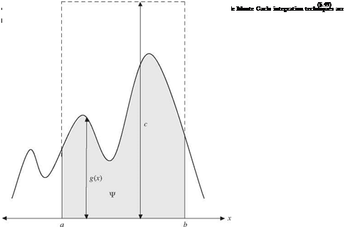
To illustrate the basic idea of the Monte Carlo integration, consider a simple one-dimensional integration


Leave a reply