Blog Archives

Mean-Value First-Order Second-Moment (MFOSM) Method

In the first-order methods, the performance function W (X), defined on the basis of the loading and resistance functions g(XL) and h(XR), are expanded in a Taylor series at a reference point. The second – and higher-order terms in the series expansion are truncated, resulting in an approximation involving only the first two statistical moments of the variables. This simplification greatly en­hances the practicality of the first-order methods because, in many problems, it is rather difficult, if not impossible, to find the PDF of the variables, whereas it is relatively simple to estimate the first two statistical moments. The pro­cedure is based on the first-order variance estimation (FOVE) method, which is summarized below...

read more

Computer Models

Many computer models have been developed for calculating rainfall runoff. Examples include the U. S. Army Corps of Engineers HEC-HMS model, the NRCS TR-20 model, and the FHWA-funded HYDRAIN system. As with all computer models, the accuracy and validity of the output can be only as accurate and valid as the input. The input and output data must be carefully inspected by a capable and practiced user to ensure valid results. (See D. R. Maidment, Handbook of Hydrology, McGraw-Hill, 1993; and Highway Drainage Guidelines, Vol. 2, AASHTO, 1999.)

Example: Time of Concentration, Rainfall Intensity, and Design Discharge. A grassy roadside channel runs 500 ft (152 m) from the crest of a hill. The area contributing to the flow is 324 ft (98 m) wide and is made up of 24 ft (7...

read more

Double adjustment

Actually all modern radiators are equipped with such comfortable device as a regulator, allowing to adjust temperature «under», and even absolutely to block access of the heat-carrier to one of radiators, without mentioning system as a whole. But as a whole read more

Method after AASHTO T 305-97

The U. S. method of mastic draindown testing has been described in the standard AASHTO T 305-97. It is used for porous asphalt mixes (also called open-graded friction course [OGFC]) and SMA mixes. Test parameters are shown in Table 8.2.

Samples of the mix are placed in wire baskets (Figure 8.3). For SMA mixes equal to and larger than 9.5 mm maximum aggregate size, the basket should have

6.3 mm holes in the mesh, and for 0/4.75 mm SMA mixes, the holes should be 2.36 mm.

8.2.3 Methods after EN 12697-18

The two methods of draindown testing that are given in the European standard EN 12697-18 are the method with a basket and Schellenberg’s method. The method with a basket after EN 12697-18 (Part 1) is mainly used for draindown testing of porous asphalt...

read more

Direct Integration Method

Direct Integration Method Подпись: dr dt Подпись: (4.11a) (4.11b)

From Eqs. (4.1) and (4.4) one realizes that the computation of reliability requires knowledge of the probability distributions of the load and resistance or of the performance function W. In terms of the joint PDF of the load and resistance, Eq. (4.1) can be expressed as

Direct Integration Method Подпись: (4.12a) (4.12b)

in which f R L(r, t) is the joint PDF of random load L and resistance R, r and t are dummy arguments for the resistance and load, respectively, and (r1, r2) and (t1, t2) are the lower and upper bounds for the resistance and load, respectively. The failure probability can be computed as

This computation of reliability is commonly referred to as load-resistance interference.

Подпись: 150

TABLE 4.1 Reliability Formulas for Selected Distributions


Distribution
of W


Coefficient of

v...

read more

Estimation of Time of Concentration

The time of concentration or rainfall duration is equivalent to the length of time it takes for the runoff to travel from the most remote point of the watershed to the point of solution. This assumes that there is a uniform rate of rainfall over the entire water­shed resulting in the maximum flow at the point being investigated. The total time of concentration is comprised of three distinct components: overland flow time, shallow concentrated flow time, and concentrated flow time.

Overland flow is thought to occur for no more than 300 ft (91 m) and perhaps even less. The overland flow time may be approximated by the curves in Fig 5.2. It is based on the following equation:

Подпись: (5.4)T = 1.8(1.1 – C)(L)1/2 o [N(100)]1/3

where To = overland flow travel time, min C = runoff coefficient L = overland tr...

read more

Original Schellenberg’s Method

A method of mastic draindown testing was published in 1986 by Kurt Schellenberg and Wolfgang von der Weppen (Schellenberg and Weppen, 1986). Their original method, which consisted of warming up a sample of SMA mix placed in a glass beaker, is summarized in Table 8.1.

TABLE 8.1

Parameters of Draindown Testing according to Schellenberg’s Method

Number of samples 1

Test temperature 170°C ± 1°C

Sample weight 1000-1100 g

Test time duration 60 ± 1 minutes

Test procedure 1. Warm-up an empty beaker in an oven at test temperature, take it out and

weigh it, and put it into the oven.

2. Mix SMA components.

3. Remove the beaker from the oven, quickly put a prepared mix into the beaker, and weigh them altogether.

4. Place the beaker with the mix in the oven for 60 ± 1 minutes.

5...

read more

Performance Functions and Reliability Index

In reliability analysis, Eq. (4.3) alternatively can be written in terms of a per­formance function W (X) = W (XL, XR) as

ps = P [W(Xl, Xr) > 0] = P [W(X) > 0] (4.4)

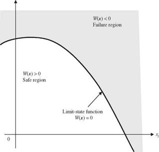
in which X is the vector of basic stochastic variables in the load and resistance functions. In reliability analysis, the system state is divided into the safe (sat­isfactory) set defined by W (X) > 0 and the failure (unsatisfactory) set defined by W (X) < 0 (Fig. 4.1). The boundary that separates the safe set and failure set is a surface, called the failure surface, defined by the function W(X) = 0, called the limit-state function. Since the performance function W(X ) defines the condition of the system, it is sometimes called system-state function.

Xk

Performance Functions and Reliability Index

Figure 4...

read more

Finding Rafter Length: Examples

Breaking the process of cutting rafters into the four basic characteristics described in this chapter helps to organize the task, but it is still a complicated process. Probably the best way to learn is to work through the steps in figuring individual rafters. The following illustration is an example of a roof that has a number of different rafters and a ridge board identified. Nine additional examples explain how to find the lengths for these rafters and ridge board based on the illustration.


Finding Common Rafter Length – Example 1 on Roof Example Illustration

The roof span at this area is 28′-0", making the run equal to У2 the span of 14′-0" minus half the thickness of the ridge board (3/4"). That makes the adjusted run 13′-111/4"...

read more

Finish Carpentry

Many manufactured composite board prod­ucts designed for interior use contain urea – formaldehyde binders. They outgas form­aldehyde for many months and contribute significantly to the indoor pollution level. In standard construction, these interior-grade

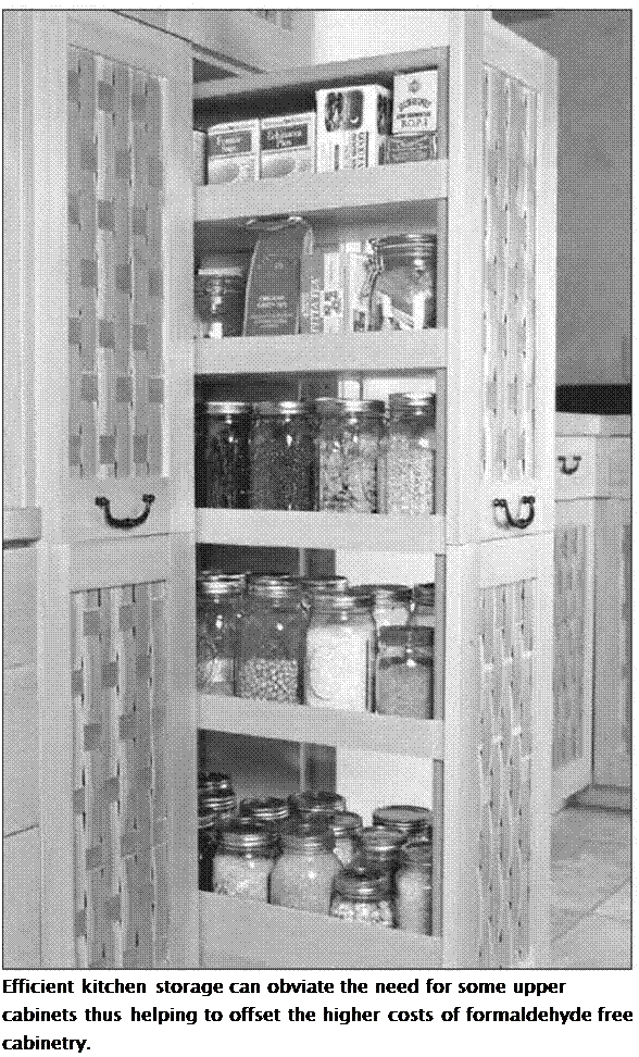
Подпись:composites are used in many finish applica­tions including cabinetry, molding, shelving, and trim. They should not be used in a healthy home. The following maybe specified:

• No sheetgoods or trim pieces containing urea-formaldehyde shall be used.

• Exposed interior finish wood shall be comprised of solid wood and finished with a low-VO C finish as specified in Division 9.

• Where sheet goods are used, choose one of the low-emission boards listed in the section on cabinets, or exterior-grade ply­wood that has been aired out, thorou...

read more