Category Hydrosystems Engineering Reliability Assessment and Risk Analysis

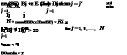
In a WLA problem, one of the most essential requirements is the assurance of a minimum concentration of dissolved oxygen (DO) throughout the river system in an attempt to maintain desired levels of aquatic biota. The constraint relating the response of DO to the additional of in-stream waste generally is defined by the Streeter-Phelps equation (Eq. 8.60) or its variations (ReVelle et al., 1968; Bathala et al., 1979). To incorporate water-quality constraints into the model formulation, a number of control points are placed within each reach of the river system under investigation. By using the Streeter-Phelps equation, each control point and discharge location becomes a constraint in the LP model, providing a check on water-quality at that location. In a general framework, a typical water quality constraint would be as follows:

Пі Пі

®ijLj + j < Rt

j=1 j=1

where

‘m-1 E[ bt, t+i I dn d=j

(8A.2)

(8A.3)

d=j

ni-1 Lo Qo П be, e+i t=j

k= j

k=ni – p+1

p=2 г=1

(8A.4)

(8A.5)

and

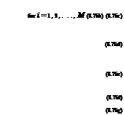
in which M is the total number of control points, Пі is the number of discharg­ers upstream of the control point i, K“ and Kdd are, respectively, the reareation and deoxygenation coefficients (days-1) in the reach, L0, Q0, and D0 are the upstream waste concentration (mg/L BOD), flow rate (ft3/s), and DO deficit (mg/L), respectively, Ddi, Ldi, and qm are the DO deficit (mg/L), waste concen­tration (mg/L BOD), and effluent flow rate (ft3/s) from each discharge location, respectively, xdi і is the distance (miles) between discharge location and control point i, and Udi is the average stream velocity (mi/day) in reach ni. Ri repre­sents the allowable DO deficit at the control point i, available for utilization of water discharge (mg/L). It should be noted that in addition to each control point i, water quality is also checked at each discharge location ni.

8.1
A city in an alluvial valley is subject to flooding. As a matter of good fortune, no serious floods have taken place during the past 50 years, and therefore, no flood – control measure of any significance has been taken. However, last year a serious flood threat developed; people realized the danger they are exposed to, and a flood investigation is under way.

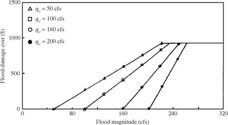
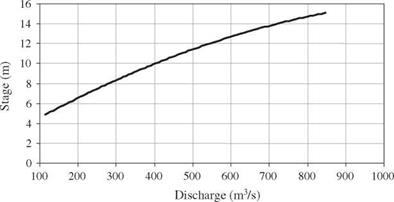
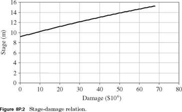
From the hydrologic flood frequency analysis of past streamflow records and hydrometric surveys, the discharge-frequency curve, rating curve, and damage curve under nature condition are derived and shown in the table below and Figs. 8P.1 and 8P.2, respectively. Also, it is known that the flow-carrying capacity of existing channel is 340 m3/s.

T (years) 2 5 10 20 50 100 200 500 1000

Q (m3/s) 255 340 396 453 510 566 623 680 736

Three flood-control alternatives are considered, and they are (1) construction of a dike system throughout the city that will contain a flood peak of 425 m3/s but will fail completely if the river discharge is higher, (2) design of an upstream permanent diversion that would divert up to 85 m3/s if the upstream inflow dis­charge exceeds existing channel capacity of 340 m3/s, and (3) construction of a detention basin upstream to provide a protection up to a flow of 425 m3/s.

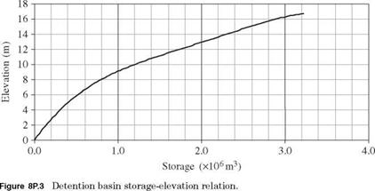
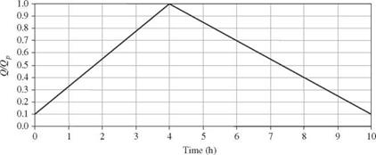
The detention basin will install a conduit with a maximum flow capacity of 340 m3/s. Assume that all flow rates less than 340 m3/s will pass through the conduit without being retarded behind the detention basin. For incoming flow rate between 340 and 425 m3/s, runoff volume will be stored temporally in the detention basin so that outflow discharge does not exceed existing downstream channel capacity. In other words, inflow hydrograph with peak discharge exceed­ing 425 m3/s could result in spillway overflow, and hence the total outflow dis­charge would be higher than the channel capacity. The storage-elevation curve at the detention basin site and normalized inflow hydrograph of different return

periods are shown in Figs. 8P.3 and 8P.4, respectively. The flow capacities of the conduit and spillway can be calculated, respectively, by

Conduit: Qc = 159h05

Spillway: Qs = 67.0(h — hs)15

where Qc and Qs are conduit and spillway capacity (in m3/s), respectively, h is water surface elevation in detention basin (in m) above the river bed, and hs is elevation of spillway crest (in m) above the river bed.

To simplify the algebraic manipulations in the analysis, the basic relations between stage, discharge, storage, and damage are derived to fit the data:

(i) Stage discharge: Q = 8.77 + 7.761 H + 3.1267H2

(ii) Stage damage: D = Max(0, -54.443 + 2.8446H + 0.34035H2)

(iii) Storage elevation: S = 0.0992 + 0.0021h + 0.011h2

h > 0; S = 0, otherwise

in which Q is flow rate in channel (m3/s), H is channel water stage (m), D is flood damage ($106), S is detention basin storage (106 m3), and h is water level in detention basin above channel bed (m).

With all the information provided, answer the following questions:

(a) Develop the damage-frequency curve for the natural condition.

(b) What is the height of spillway crest of the detention basin above the river bed?

(c) Develop the damage-frequency curves as the results of each of the three flood control measures.

(d) Rank the alternatives based on their merits on the flood damage reduction.

8.2 Refer to Problem 8.1 and consider the alternative of building a levee system for flood control. It is known that the capital-cost function for constructing the levee system is

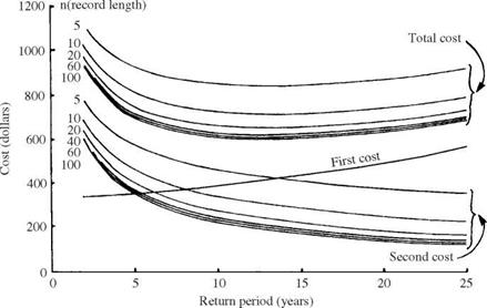
FC(Y) = 1.0 + 0.6(Y – 7) + 0.05(Y – 7)3 in which Y is the height of levee, and FC(Y) is the capital cost (in million dollars). Suppose that the service period of the levee system is to be 50 years and the interest rate is 5 percent. Determine the optimal design return period such that the annual total expected cost is the minimum.

8.3 Consider a confined aquifer with homogeneous soil medium. Use the Thiem equa­tion and the linear superposition principle (see Problem 2.30) to formulate a steady-state optimal groundwater management model for the aquifer system sketched in Fig. 8P.5. The management objective is to determine the maximum total allowable pumpage from the three production wells such that the drawdown of piezometric head at each of the five selected control point would not exceed a specified limit.

+ І

(a) Formulate a linear programming model for the groundwater system as shown in Fig. 8P.5.

(b) Suppose that the radius of influence of all pump wells is 700 ft (213 m) and that the aquifer transmissivity is 5000 gal/day/ft (0.00072 m2/s). Based on the information given in Fig. 8P.5, solve the optimization model formulated in part (a).

8.4 Consider that the soil medium is random and that the transmissivity has a log­normal distribution with mean value of 5000 gal/day/ft and a coefficient of vari­ation of 0.4. Construct a chance-constrained model based on Problem 8.3, and solve the chance-constrained model for a 95 percent compliance reliability of all constraints.

8.5 Modify the formulation in Problem 8.3, and solve the optimization model that maximizes the total allowable pumpage in such a way that the largest drawdown among the five control points does not exceed 10 ft.

8.6 Develop a chance-constrained model based on Problem 8.5, and solve the model for a 95 percent compliance reliability of all constraints.

8.7 Based on the chance-constrained model established in Problem 8.6, explore the tradeoff relationship among the maximum total pumpage, compliance reliability, and the largest drawdown.

8.8 Modify the formulation in Problem 8.6 to develop a chance-constrained manage­ment model for the hypothetical groundwater system that maximizes the total allowable pumpage while satisfying the desired lowest compliance reliability for all constraints. Furthermore, solve the model for the hypothetical system shown in Fig. 8P.5 with the lowest compliance reliability of 95 percent.

8.9 In the design of a water supply system, it is general to consider a least-cost system configuration that satisfies the required water demand and pressure head at the demand points. The cost of the system may include the initial investment for the components (e. g., pipes, tanks, valves, and pumps) and the operational costs. The optimal design problem, in general, can be cast into

Minimize Capital cost + energy cost subject to (1) Hydraulic constraints

(2) Water demands

(3) Pressure requirements

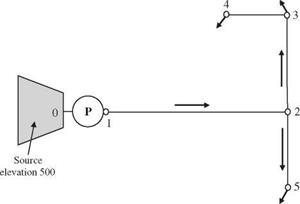
Consider a hypothetical branched water distribution system as shown in Fig. 8P.6. Develop a linear programming model to determine the optimal combination of cast iron pipe length of various commercially available pipe sizes for each branch. The objective is to minimize the total pipe cost of the system, subject to water demand and pressure constraints at all demand points. The new cast iron pipes of all sizes have the Hazen-Williams roughness coefficient of 130. The cost of pumping head is $500/ft, and the pipe costs for available pipe sizes are listed below

To this hypothetical system, the required flow rate and water pressure at each demand node are

[1] Obtain the probability paper corresponding to the distribution one wishes to fit to the data series.

[2] Identify the sample data series to be used. If high-return-period values are of interest, either the annual maximum or exceedance series can be used. If low-return-period values are of interest, use an annual exceedance series.

[3] Rank the data series in decreasing order, and compute exceedance probabil­ity or return period using the appropriate plotting-position formula.

[4] Plot the series, and draw a best-fit straight line through the data. An eye­ball fit or a mathematical procedure, such as the least-squares method, can be used. Before doing the fit, make a judgment regarding whether or not to include the unusual observations that do not lie near the line (termed outliers).

[5] Compute the sample mean x, standard deviation ax, and skewness coefficient Yx (if needed) for the sample.

[6] Inability to handle distributions with a large skewness coefficient. Table 4.2 indicates that the discrepancy of the failure probability estimated by the MFOSM method for a lognormally distributed performance function becomes larger as the degree of skewness increases. This mainly due to the fact that the MFOSM method incorporates only the first two moments of the random parameters involved. In other words, the MFOSM method simply ignores any moments higher than the second order. Therefore, for those random variables having asymmetric PDFs, the MFOSM method cannot capture such a feature in the reliability computation.

[7] Generally poor estimations of the mean and variance of nonlinear functions. This is evident in that the MFOSM method is the first-order representation

[8] Inappropriateness of the expansion point. In reliability computation, the con­cern often is those points in the parameter space that fall on the failure sur­face or limiting-state surface. In the MFOSM method, the expansion point is located at the mean of the stochastic basic variables that do not necessar­ily define the critical state of the system. The difference in expansion points and the resulting reliability indices between the MFOSM and its alternative, called the advanced first-order, second-moment method (AFOSM), is shown in Fig. 4.3.

[9] The seed X0 can be chosen arbitrarily. If different random number sequences are to be generated, a practical way is to set X0 equal to the date and time when the sequence is to be generated.

2. The modulus m must be large. It may be set conveniently to the word length of the computer because this would enhance computational efficiency. The computation of {aX + c}(mod m) must be done exactly without round-off errors.

3. If modulus m is a power of 2 (for binary computers), select the multiplier a so that a(mod 8) = 5. If m is a power of 10 (for decimal computers), pick a such that a(mod 200) = 21. Selection of the multiplier a in this fashion, along with the choice of increment c described below, would ensure that the random number generator will produce all m distinct possible values in the sequence before repeating itself.

4. The multiplier a should be larger than */m, preferably larger than m/100, but smaller than m -*Jm. The best policy is to take some haphazard constant to be the multiplier satisfying both conditions 3 and 4.

5. The increment parameter c should be an odd number when the modulus m is a power of 2 and c should not be a multiple of 5 when m is a power of 10.

[10] Obtain the eigenvector matrix and diagonal eigenvalue matrix of the corre­lation matrix Rx or covariance matrix Cx.

[11] Generate K independent standard normal random variates z’ = (z1, z’2

zK У.

[12] Compute the correlated normal random variates X by Eq. (6.36).

[13] Select fx (x) defined over the region of the integral from which n random variates are generated.

[14] Compute g(xi)/fx(xi), for i = 1, 2,…, n.

[15] Calculate the sample average based on Eq. (6.60) as the estimate for G.

[16] Generate K independent standard normal random variates z’ = (z-, z2,…, z’K), and compute the corresponding directional vector e = z’/|z’|

[17] Transform stochastic variables in the original X-space to the independent standard normal Z ‘-space.

The WLA problem, by nature, is a multiobjective problem involving several conflicting objectives. The treatment-equity constraint (Eq. 8.59c) is incorpo­rated for the purpose of fairness. Without it, any attempt to maximize waste discharge (or to minimize treatment cost) could result in allocating large quan­tities ofwaste to the upstream users, whereas the downstream discharges could be required to treat their effluent at levels of maximum possible efficiency. This is especially true for slow-moving streams. Several articles have discussed the importance of equity considerations in WLA problems (Gross, 1965; Loucks et al., 1967; Miller and Gill, 1976; Brill et al., 1976).

In general, as the requirement for an equity measure (or fairness) is raised, the total waste discharge to the stream system would be reduced. This will be in direct conflict with the maximization of waste discharge associated with the minimization of treatment cost. Furthermore, from the preserving stream water-quality viewpoint, setting a higher water-quality standard is more desir­able. However, such an objective cannot be achieved without increasing waste treatment cost. Therefore, the objectives of preserving water quality and of
enhancing economic efficiency are in conflict each other. Lastly, as the require­ment of reliability in complying with the water-quality standard is raised, the total waste load that can be discharged expectedly would have to be reduced. Therefore, the task of solving WLA problems is multiobjective.

From the preceding discussions, four objective functions can be considered in WLA modeling: (1) maximization of the total waste load, (2) minimization of differences in treatment levels among waste dischargers, (3) maximization of allowable in-stream DO concentration, and (4) maximization of the water – quality standard compliance reliability. The first objective Z1 can be formulated as Eq. (8.59a), which is repeated here as

N

Maximize Z1 = (Bj + Dj)

j=i

For a stream system involving multiple waste dischargers, the difference in required treatment levels generally would vary. To collapse different values of equity measure into a single representative indicator, the worst case associated with the largest differences can be used. With that, the second objective can be expressed as

where 5max is a new decision variable for the equity measure representing the largest difference in treatment levels among waste dischargers.

The third objective considered is the maximization of the lowest allowable DO concentration level that should be maintained in the stream environment. This objective can be expressed as

Maximize Z3 = DO^

in which the new decision variable DOsmtdin is the minimum required DO standard in the stream.

Similar to the differences in treatment levels, the water-quality compliance reliability at different control points will not be uniform. To use a single repre­sentative measure of compliance reliability for the entire system, a conservative view of looking at the lowest reliability was applied. The objective is to maximize this lowest compliance reliability amin as

Maximize Z4 = amin = min[a1, a2,…, aM ] (8.71)

By the definitions of DO^^in and amin, the chance constraints for water-quality compliance (Eq. 8.59b) can be modified as

(8.72)

The corresponding deterministic equivalent of Eq. (8.72) can be expressed as

П ni

(®ij) Bj + E E (Vj Dj + DOmtdn j=1 j=1

+ Fz-1(amin)V(B, D)C (&i, П)(B, D) < Ri (8.73)

in which R i = DOsat – E (aoi).

Note that the original objective given in Eq. (8.71) is to maximize amin. How­ever, under the assumption that the standardized left-hand sides of the water – quality constraints are continuous and unimodal random variables, the deci­sion variable amin would have a strictly increasing relationship with Fz_1(amin). Therefore, maximization of amin is then equivalent to maximizing Fz_1(amin). By letting zmin = Fz_1(amin), Eq. (8.71) can be written as

Maximize Z4 = zmin (8.74)

Note that the decision variable zmin is unrestricted in sign. The objective of maximizing the lowest compliance reliability is equivalent to minimizing the highest water-quality violation risk.

The preceding multiobjective WLA problem can be solved by various tech­niques described in the references cited in Sec. 8.1.2. In the following, the con­straint method is used by which the preceding multiobjective WLA problem is expressed as

Maximize zmin

subject to

and nonnegativity constraints for the decision variables, except for zmin. In Eqs. (8.75e-g), the right-hand sides Z, ZO, and Z3 are the values of the objective functions 1, 2, and 3, respectively, which are to be varied parametrically.

Using the same hypothetical stream system as shown in Fig. 8.21 and the corresponding data, the solution to this multiobjective WLA model by the con­straint method yields a series of tradeoff curves among the various objectives. Figures 8.22 through 8.24 show the tradeoffs among three objectives for a given

minimum DO standard concentration. As can be seen for a specified minimum DO standard and total waste load, the largest water-quality violation risk de­creases as the maximum difference in treatment equity increases. An increase in the treatment equity measure by 5max implies a larger tolerance for the

unfairness in the treatment requirement among waste dischargers. As the level of the minimum required DO standard is raised, the set of tradeoff curves moves upward. To show the tradeoffs for different minimum DO standard, Figs. 8.25 and 8.26 are plotted for the risk of water-quality standard violation, treatment equity, and water-quality standard while the total waste load to the stream system is fixed at some specified levels.

Deterministic waste-load allocation model. Although any number of pollutants may be considered in the overall quality management of a river system, in this example, application a biochemical oxygen demand-dissolved oxygen (BOD-DO) water-quality model is considered.

In LP format, the deterministic WLA model considered herein can be written as

N

Maximize ^^( Bj + Dj)

j=i

subject to

1. Constraints on water quality:

aoi + ®ij Bj + ^ ttij Dj < DOsat – DOfd for i = 1,2,…, M (8.59b)

j=1 j=1

2.

Constraints on treatment equity:

3. Constraints on treatment efficiency:

Bj

e-j < 1 – T <e j

j

where Bj, Dj, and Ij are the effluent waste concentrations (mg/L BOD), ef­fluent DO deficit concentration (mg/L), and raw waste influent concentration (mg/L BOD) at discharge location j, respectively, and N is the total number of waste dischargers. The LHS coefficients aoi, ®ij, and Uij in Eq. (8.59b) are
the technological transfer coefficients relating impact on DO concentrations at downstream locations i resulting from the background waste and waste input at an upstream location j. These technological transfer coefficients are functions of water-quality parameters such as reaeration and deoxygenation rates, flow velocity, etc. DOistd and DOisat represent the required DO standard and saturated DO concentration at control point i, respectively. Finally, Ea is the allowable dif­ference (i. e., equity) in treatment efficiency between two waste dischargers, and e_j and e j are the lower and upper bounds of waste-removal efficiency for the j th discharger, respectively. The importance of incorporating the treatment equity in the WLA problems is discussed by many researchers (Gross, 1965; Loucks et al., 1967; Miller and Gill, 1976; Brill et al., 1976; Chadderton et al., 1981).

The water-quality constraint relating the response of DO to the effluent waste can be defined by water-quality models such as the Streeter-Phelps equation (Streeter and Phelps, 1925) or its variations (Dobbins, 1964; Krenkel and Novotny, 1980). To demonstrate the proposed methodologies, the original Streeter-Phelps equation is used herein to derive the water-quality constraints. Expressions for &ij and Uij, based on the Streeter-Phelps equation, are shown in Appendix 8A. The Streeter-Phelps equation for DO deficit is given as follows:

Dx = TKdL0, (e-KdX/U – e-K“x/U) + Doe-Kax/U (8.60)

where Dx is the DO deficit concentration (mg/L) at stream location x (mi), Kd is the deoxygenation coefficient for BOD (days-1), Ka is the reaeration-rate coefficient (days-1), L0 is the BOD concentration at the upstream end of the reach (that is, x = 0), D0 is the DO deficit concentration at the upstream end of the reach, and U is the average streamflow velocity in the reach (mi/day).

Chance-constrained waste-load allocation model. The deterministic WLA model presented in Eqs. (8.59a-d) serves as the basic model for deriving the stochastic WLA model. Considering the existence of uncertainty within the stream envi­ronment, the water-quality constraints given by Eq. (8.59b) can be expressed probabilistically as

Пі Пі j

aoi + X) ©ij Bj + 53 Uij Dj < DOsat – DOfd> ai for і = 1,2,…, M

j=1 j=1 )

(8.61)

Based on Eq. (8.53), the deterministic equivalent of Eq. (8.60) can be derived as

(8.62)

in which Ri = DOSat – DOfd – E(a0i), (B, D) is the column vector of BOD and DO deficit concentrations in waste effluent, and C (©i, Qi) is the covariance matrix associated with the technological transfer coefficients in the ith water – quality constraint, including a0i. The stochastic WLA model to be solved consists of Eqs. (8.58a), (8.62), (8.58c), and (8.58d).

Assessments of statistical properties of random technological coefficients. To solve the stochastic WLA model, it is necessary to assess the statistical properties of the random LHS in the chance-constraint Eq. (8.62). As shown in Appendix 8A, the technological transfer coefficients &ij and Uij are nonlinear functions of the stochastic water-quality parameters that are cross-correlated among them within each stream reach and spatially correlated between stream reaches. Furthermore, the complexities of the functional relationships between these transfer coefficients and the water-quality parameters increases rapidly as the control point moves downstream. Hence the analytical derivation of the statistical properties of &ij and Uij becomes a formidable task given even a small number of reaches. As a practical alternative, simulation procedures may be used to estimate the mean and covariance structure of the random techno­logical coefficients within a given water-quality constraint.

The assumptions made in the Monte Carlo simulation to generate water – quality parameters in all reaches of the stream system are as follows: (1) The representative values for the reaeration coefficient, deoxygenation coefficient, and average flow velocity in each reach are second-order stationary; i. e., the spatial covariance functions of water quality-parameters are dependent only on the “space lag” or separation distance; (2) correlation between the reaeration coefficient and average flow velocity exists only within the same stream reach; (3) background DO and BOD concentrations at the upstream end of the entire stream system are independent of each other and of all other water-quality parameters; and (4) all water-quality parameters follow a normal distribution.

In the simulation, variance-covariance matrices representing the spatial cor­relation of a water-quality parameter can be derived from the variogram models (Journel and Huijbregts, 1978) in the field of geostatistics. Three commonly used variogram models are:

1. Transitive variogram model:

(8.63)

2. Spherical variogram model:

(8.64)

3.

Gaussian variogram model:

in which Cov(|h|) represents the value of covariance between two measure­ments of the same water-quality parameter separated by a distance h | apart, ho is the length of zone of influence, and a2 is the variance of the water – quality parameter within a given reach. The value of correlation coefficient p(|h|) can be calculated as p(|h|) = Cov(|h|)/a2. When the distance between reaches exceeds ho, the value of the covariance function goes to zero, and the corresponding correlation coefficient is zero as well. Graphically, the three variogram models are shown in Fig. 8.18.

To illustrate the concept, consider the water-quality parameters’ reaeration coefficient Ka and average flow velocity U. From the variogram models, the correlation matrix for the two parameters can be constructed as follows:

in which Ka = (Ka, i, Ka2,…, Ka N) and U = (Ui, U2,…, UN) are vectors of the reaeration coefficient and average velocity in each stream reach, respec­tively (see Fig. 8.19). In Eq. (8.66), R(Ka, Ka), R(Ka, U), R(U, U) are N x N square symmetric correlation matrices, with N being the number of stream reaches in the WLA model. Submatrices R(Ka, Ka) and R(U, U) define the spa­tial correlation of Ka and U between the reaches, whereas submatrix R(Ka, U) defines the cross-correlation between Ka and U within the same reach. Under assumption 2 previously mentioned, the submatrix R(Ka, U) is a diagonal ma­trix. For water-quality parameters that are not cross-correlated with other pa­rameters but are spatially correlated, the associated correlation matrix has a form similar to R(U, U). For parameters that are spatially independent, their correlation matrices are in the form of an identify matrix. Once the correlation matrix of normal stochastic parameters within a reach and between reaches is established according to the specified variogram model, generation of stochastic water-quality parameters can be obtained easily by the procedures for gener­ating multivariate random variates described in Sec. 7.5.2.

In summary, the simulation for generating spatially and cross-correlated water-quality parameters can be outlined as the follows:

1. Select an appropriate variogram model for a given water-quality parameter, and construct the corresponding covariance matrix C or correlation matrix R.

2. Apply procedures described in Sec. 7.5.2 to obtain the values of the water – quality parameter for each reach in the WLA model.

3. Repeat steps 1 and 2 for all water-quality parameters.

For each set of the water-quality parameters generated by steps 1 through 3, the values of the technological coefficients are computed. Based on the simu­lated values, the mean and covariance matrices of the random technological coefficients for each water-quality constraint are calculated and used in solving the stochastic WLA problem. The simulation procedure described in this sub­section to account for spatial correlation is called unconditional simulation in the field of geostatistics (Journel and Huijbregts, 1978).

Technique for solving an optimal stochastic WLA model. The deterministic WLA model presented previously follows an LP format and can be solved using the simplex algorithm. However, the deterministic equivalents of the chance – constrained water-quality constraints are nonlinear. Thus the problem is one of nonlinear optimization, which can be solved by various nonlinear programming techniques mentioned in Sec. 8.1.2.

In this example, linearization of the chance-constrained water-quality constraints is done, and the linearized model is solved iteratively using the LP simplex technique. More specifically, the algorithm selects an assumed solution to the stochastic WLA model that is used to calculate the value of the nonlinear terms in Eq. (8.62). The nonlinear terms then become constants and are moved to the RHS of the constraints. The resulting linearized water-quality constraints can be written as

E(®ij)Bj + E(Qij)Dj < Щ – F-1(at) (B, t»tC(&t, )(B, D)

j=1 J =1

(8.67)

in which B and D are assumed solution vectors to the stochastic WLA model.

The linearized stochastic WLA model, replacing Eq. (8.62) by Eq. (8.67), can be solved using LP techniques repeatedly, each time updating the previous

solution values with those obtained from the current iteration, resulting in new values for the RHS. The procedure is repeated until convergence criteria are met between any two successive iterations. A flowchart depicting the procedures is given in Fig. 8.20. Of course, alternative stopping rules could be incorporated in the algorithm to prevent excessive iteration during the computation. Prior to the application of these solution procedures, an assumption for the distribution of the random LHS must be made to determine the appropriate value for the term Fz(ai) in Eq. (8.67).

Owing to the nonlinear nature of the stochastic WLA model, the global op­timum solution, in general, cannot be guaranteed. It is suggested that a few runs of the solution procedure with different initial solutions be carried out to ensure that the model solution converges to the overall optimum. A reasonable initial solution is to select the waste effluent concentration for each discharger associated with the upper bounds of their respective treatment levels. By doing so, the initial solution corresponds to waste discharge at their respective lower

limits. If the stochastic WLA solution is infeasible during the first iteration, it is likely that the feasible solution to the stochastic WLA problem does not exist. Hence time and computational effort could be saved in searching for an optimal solution that might not exist.

Numerical example. The preceding chance-constrained WLA model is applied to a six-reach example shown in Fig. 8.21. The means and standard deviations for the water-quality parameters in each reach are given in Tables 8.5 and 8.6 based on the data reported in the literature (Churchill et al., 1962; Chadderton et al., 1982; Zielinski, 1988).

To assess the mean and correlation matrix of the random technological co­efficients in the water-quality constraints, the Monte Carlo simulation proce­dure described in Sec. 6.5.2 is implemented to generate multivariate normal water-quality parameters. Different numbers of simulation sets are generated to examine the stability of the resulting means and covariance matrix of the technological coefficients. It was found that the statistical properties of ©ij and Uij become stable using 200 sets of simulated parameters. In the exam­ple, a positive correlation coefficient of 0.8 between the reaeration coefficient and average flow velocity is used. Both normal and lognormal distributions are assumed for the random LHS of the water-quality constraints

Пі Пі

a0i + 53 ©i> + 53 ^ij Dj (8.68)

j=1 j=1

in Eq. (8.67). Various reliability levels ai ranging from 0.85 to 0.99 for the water-quality constraints are considered.

In the example, the length of each reach in the system is 10 mi, and the spatial correlation of representative water-quality parameter values between two reaches is computed based on the separation distance between the centers of the two reaches. To examine the effect of spatial correlation structure on the optimal waste-load allocation, two zones of influence (ho = 15 mi and ho = 30 mi) along with the three variogram models, Eqs. (8.63) through (8.65), are used. A value of ho = 15 mi implies that the water-quality parameters in a given reach are spatially correlated only with the two immediate adjacent reaches. For ho = 30 mi, the spatial correlation extends two reaches upstream and downstream of the reach under consideration. The optimal solutions to the stochastic WLA problem under these various conditions are presented in Tables

8.7 and 8.8.

Examining Tables 8.7 and 8.8, the maximum total BOD discharge, under a given spatial correlation structure, reduces as the reliability of water-quality constraints increases. This behavior is expected because an increase in water – quality compliance reliability is equivalent to imposing stricter standards on water-quality assurance. To meet this increased water-quality compliance re­liability, the amount of waste discharge must be reduced to lower the risk of water-quality violation at the various control points. When continuing to in­crease the required reliability for the water-quality constraints, at some point these restrictions could become too stringent, and feasible solutions to the prob­lem are no longer obtainable.

From Tables 8.7 and 8.8, using a lognormal distribution for the LHS of water – quality constraints yields a higher total BOD discharge than that under a nor­mal distribution when the performance reliability requirement is 0.85. How­ever, the results reverse themselves when reliability requirements are greater than or equal to 0.90. This indicates that the optimal solution to the stochastic WLA model depends on the distribution used for the LHS of the water-quality constraints. From the investigation of Tung and Hathhorn (1989), a lognor­mal distribution was found to best describe the DO deficit concentration in a single-reach case. In other words, each term of the LHS in the water-quality

constraints could be considered as a lognormal random variable. Therefore, the LHS is the sum of correlated lognormal random variables. For the first two or three reaches from the upstream end of the system, the distribution of the LHS may close to lognormal because the number of terms in the LHS is few. How­ever, considering the control point for farther-downstream reaches, the number of terms in the LHS increases, and the resulting distribution may approach to normal from the argument of the central limit theorem. Since the true distribu­tion for the LHS of water-quality constraints is not known, it is suggested that different distributions be used for model solutions and that the least amount of total BOD load be applied for implementation.

Furthermore, the impacts of the extent of the spatial correlation of the water – quality parameters (represented by the length of ho) and the structure (repre­sented by the form of the variogram) on the results of the stochastic WLA model also can be observed. When ho = 15 mi, where the spatial correlation of the water-quality parameters extends only one reach, the maximum allowable total BOD load, for all three variogram models, is higher than that of spatially independent case. When the spatial correlation extends over two reaches (that is, ho = 30 mi), use of transitive and spherical variogram models results in lower maximum total BOD loads than that of the spatially independent case, whereas use of a Gaussian variogram yields a higher total BOD load. The model results using a transitive variogram are very similar to those of a spherical model.

As a final comment on the computational aspects of the proposed technique for solving the stochastic nonlinear WLA model formulated in this study, it was observed that the iterative technique proposed takes three to five iterations to converge for all the cases investigated. Therefore, the proposed solution proce­dure is quite efficient in solving the stochastic WLA model.

Water-quality management is the practice of protecting the physical, chemi­cal, and biologic characteristics of various water resources. Historically, such efforts have been guided toward the goal of assessing and controlling the im­pacts of human activities on the quality of water. To implement water-quality management measures in a conscientious manner, one must acknowledge both the activities of the society and the inherently random nature of the stream environment itself (Ward and Loftis, 1983). In particular, the environments in which decisions are to be made concerning in-stream water-quality manage­ment are inherently subject to many uncertainties. The stream system itself, through nature, is an environment abundant with ever-changing and complex processes, both physically and biologically.

Public Law 92-500 (PL 92-500) in the United States provided impetus for three essential tasks, one of which is to regulate waste-water discharge from point sources from industrial plants, municipal sewage treatment facilities, and livestock feedlots. It also requires treatment levels based on the best available technology. However, if a stream segment is water-quality-limited, in which the waste assimilative capacity is below the total waste discharge authorized by PL 92-500, more stringent controls may be required.

For streams under water-quality-limited conditions or where effluent stan­dards are not implemented, the waste-load-allocation (WLA) problem is con­cerned with how to effectively allocate the existing assimilative capacity of the receiving water body among several waste dischargers without detrimen­tal effects to the aquatic environment. As an integral part of water-quality management, WLA is an important but complex decision-making task. The results of WLA have profound implications on regional environmental protec­tion. A successful WLA decision requires sound understanding of the physi­cal, biologic, and chemical processes of the aquatic environment and good ap­preciation for legal, social, economical, and environmental impacts of such a decision.

Much of the research in developing predictive water-quality models has been based on a deterministic evaluation of the stream environment. Attempts to manage such an environment deterministically imply that the compliance with water-quality standards at all control points in the stream system can be en­sured with absolute certainty. This, of course, is unrealistic. The existence of the uncertainties associated with stream environments should not be ignored. Thus it is more appropriate in such an environment to examine the performance of the constraints of a mathematical programming model in a probabilistic con­text. The random nature of the stream environment has been recognized in the WLA process. Representative WLA using a chance-constrained formulation can be found elsewhere (Lohani and Thanh, 1979; Yaron, 1979; Burn and McBean, 1985; Fujiwara et al., 1986, 1987; Ellis, 1987; Tung and Hathhorn, 1990).

In the context of stochastic management, the left-hand-side (LHS) coefficients of the water-quality constraints in a WLA model are functions of various ran­dom water-quality parameters. As a result, these LHS coefficients are random
variables as well. Furthermore, correlation exists among these LHS coeffi­cients because (1) they are functions of the same water-quality parameters and (2) some water-quality parameters are correlated with each other. Moreover, the water-quality parameters along a stream are spatially correlated. There­fore, to reflect the reality of a stream system, a stochastic WLA model should account for the randomness of the water-quality parameters, including spatial and cross-correlations of each parameter.

The main objective of this section is to present methodologies to solve a stochastic WLA problem in a chance-constrained framework. The randomness of the water-quality parameters and their spatial and cross-correlations also are taken into account. A six-reach example is used to demonstrate these method­ologies. Factors affecting the model solution to be examined are (1) the distri­bution of the LHS coefficients in water-quality constraints and (2) the spatial correlation of water-quality parameters.

In all fields of science and engineering, the decision-making process depends on several parameters describing system behavior and characteristics. More often than not, some of these system parameters cannot be assessed with certainty. In a system-optimization model, if some of the coefficients in the constraints

are uncertain, the compliance with the constraints, under a given set of solu­tions, cannot be ensured with certainty. Owing to the random nature of the constraint coefficients, a certain likelihood that constraints will be violated al­ways exists. The basic idea of chance-constrained methods is to find the solution to an optimization problem such that the constraints will be met with a speci­fied reliability. Chance-constrained formulations have been applied to various types of water resource problems such as groundwater quantity management (Tung, 1986), groundwater quality management (Gorelick, 1982; Wagner and Gorelick, 1987, 1989; Morgan et al., 1993; Ritzel et al., 1994) and monitoring network design (Datta and Dhiman, 1996), reservoir operation (Loucks et al., 1981; Houck, 1979; Datta and Houck, 1984), waste-load allocation (Lohani and Thanh, 1978; Fujiwara et al., 1986, 1987; Ellis, 1987; Tung and Hathhorn, 1990), water distribution systems (Lansey et al., 1989), and freshwater inflow for estuary salinity management (Tung et al., 1990; Mao and Mays, 1994). This section describes the basic properties of chance-constrained models. In the next section an application to waste-load allocation is presented for illustration.

Refer to the general nonlinear optimization problem as stated in Eqs. (8.1a-c). Consider a constraint g(x) < b, with x being a vector of decision variables. In general, decision variables x in an optimization model are controllable without uncertainty. Suppose that some of the parameters on the left-hand-side (LHS) of the constraint g(x) and/or the right-hand-side (RHS) coefficient b are subject to uncertainty. Because of the uncertainty, the compliance with the constraint under a given solution set x cannot be ensured with absolute certainty. In other words, there is a possibility that for any solution x, the constraint will be vio­lated. Consequently, the chance-constrained formulation expresses the original constraint in a probabilistic format as

P [g(x) < b] > a (8.42)

where P [ ] is the probability and a is the specified reliability for constraint compliance. Since this chance-constrained formulation involves probability, it is not mathematically operational for algebraic solution. For this reason, the deterministic equivalent must be derived. There are three cases in which the random elements in Eq. (8.42) could occur: (1) only elements ing(x) are random,

(2) only the RHS b is random, and (3) both g(x) and b are random.

The simplest case is the case 2, where only the RHS coefficient b is random. The derivation of deterministic equivalent of the chance-constraint for this case can be done as follows: The constraint can be rewritten as

P [g(x) < B] > a (8.43)

where B is a random RHS coefficient. Since Eq. (8.43) can be written as then Eq. (8.44) can be expressed as

Fb [g(x)] < 1 – « (8.45)

in which Fb [ ] is the cumulative distribution function (CDF) of random RHS B. The deterministic equivalent of the original chance-constraint Eq. (8.43) can be expressed as

g(x) < b1-a (8.46)

where, referring to Fig. 8.17, b1-a is the (1 – a)th quantile of the random RHS coefficient B satisfying P(B < b1-a) = 1 – a. If the RHS coefficient B is a normal random variable with mean цb and standard deviation ab, Eq. (8.46) can be written as

g(x) < ^b + Z1-aab (8.47)

with z1-a being the (1 – a)th standard normal quantile.

In the case that only the elements in g(x) are random and the distribution functions are known, the chance-constraint can be expressed as

P [G(x) < b] > a (8.48)

For a general nonlinear function G(x), the difficulty lies in the derivations of exact probability distribution and statistical moments of G(x) as functions of unknown decision variables. In this circumstance, statistical moments of G(x) can be estimated by uncertainty-analysis methods such as those described in Tung and Yen (2005). The assessment of the distribution for G(x) is, at best, to be made subjectively. For the sake of discussion, assume that the distribution function of G( x) is known. The deterministic equivalent of the chance-constraint Eq. (8.48) can be expressed as

FG(i>(a) > b (8.49)

where F—yia) is the ath quantile of the random G(x), which is the function of unknown decision variables x. In general, FG(X)(a) in Eq. (8.48) is a nonlinear equation of x even if G(x) is a linear function of x, as will be shown later.

The third case is when both G(x) and the RHS coefficient B are random. The chance-constraint then can be expressed as

P [G(x) – B < 0] > a (8.50)

The deterministic equivalent of Eq. (8.49) can be derived as

Fg^-b (a) > 0 (8.51)

where Fc-(1x)_B (a) is the inverse of the CDF of random G(x) – B taken on the value of a.

As a special case, consider an LP formulation as stated in Eq. (8.3) in which technological coefficients A and/or RHS coefficients b are subject to uncertainty. By imposing a reliability restriction a on the system constraints, the LP model can be transformed into the following chance-constrained formulation:

Maximize c lx (8.52a)

subject to P (Ax < b) > a (8.52b)

In a chance-constrained LP model, the elements in A, b, and c can be random variables. When the objective function coefficient Cj’s are random variables, it is common to replace them by their expected values. Consider the follow­ing three cases: (1) elements of the technological coefficient matrix (Aij’s) are random variables, (2) elements of the RHS vector Bi’s are random variables, and

(3) elements Aij and Bi are simultaneously random variables. In the following derivations, it is assumed that random technological coefficients and random RHS coefficient are correlated within a constraint and that these coefficients are uncorrelated between constraints.

Consider that the RHS of the ith constraint Bi is subject to uncertainty. Fur­thermore, assume that its distribution and statistical moments are known. In this case, the deterministic equivalent of the chance-constraint can be obtained easily from Eq. (8.46) as

n

5^aijXj < bi,1-ai for i = 1, 2,…, m (8.53)

j=1

and the constraint form remains linear.

Consider the case that the technological coefficients aij’s of the ith constraint are random. The deterministic equivalent of the chance-constraint

P (53 AijXj < bi ) >

j=1

can be derived as (Kolbin, 1977; Vajda, 1972)

n

Y. E(Aij)xj + FzHai)vXCX < bi (8.54)

j=1

where E (Aij) is an expectation of the technological coefficient Aij, Ci is an n x n covariance matrix of n random technological coefficients (Ai 1, Ai2, …, Ain) in the ith constraint, and F—1(ai) is the appropriate quantile for the ai percentage given by the CDF of standardized left-hand-side (LHS) terms. That is,

LHSi – E(LHSi) Sn=1 AijXj -£n=1 E(Aij)x}

VVar(LHSi)

If all Aij’s are independent random variables, that is, p(Aij, Aij>) = 0, for j = j’, matrix Ci is a diagonal matrix of variances of Aij. To quantify F—1(ai), the distribution of LHS must be known or assumed. Note that the LHSs in an LP model are the sum of several random variables. By the central limit theorem (see Sec. 2.6.1), the random LHS can be approximated as a normal random variable. Therefore, Eq. (8.54) can be written as

E(Aij)Xj + Ф 1(«i)y/x*Cix < bi (8.56)

j=1

with Ф( ) being the standard normal CDF. From Eq. (8.55) one realizes that when Aij’s are random, the resulting deterministic equivalents of the chance constraints are no longer linear functions of the decision variables. The chance – constrained model has to be solved by nonlinear programming algorithms. In the next subsection of application, a sequential LP algorithm is used to linearize Eq. (8.56).

Finally, when both the technological coefficients and the RHS coefficient of the ith constraint are random, the chance-constraint format, referring to Eq. (8.50), can be written as

A flood-damage-reduction plan includes measures that decrease damage by reducing discharge, stage, and/or damage susceptibility (U. S. Army Corps of Engineers, 1996). For federal projects in the United States, the objective of the plan is to solve the problem under consideration in a manner that will “… contribute to national economic development (NED) consistent with protecting the Nation’s environment, pursuant to national environmental statutes, appli­cable executive orders, and other Federal planning requirements” (U. S. Water Resources Council, 1983). In the flood-damage-reduction planning traditionally done by the U. S. Army Corps of Engineers (Corps), the level of protection pro­vided by the project was the primary performance indicator (Eiker and Davis, 1996). Only projects that provided a set level of protection (typically from the 100-year flood) would be evaluated to determine their contribution to NED, effect on the environment, and other issues. The level of protection was set without regard to the vulnerability level of the land to be protected. In order to account for uncertainties in the hydrologic and hydraulic analyses applied in the traditional method, safety factors, such as freeboard, are applied in project design in addition to achieving the specified level of protection. These safety fac­tors were selected from experience-based rules and not from a detailed analysis of the uncertainties for the project under consideration.

The Corps now requires risk-based analysis in the formulation of flood – damage-reduction projects (Eiker and Davis, 1996). In this risk-based analysis, each of the alternative solutions for the flooding problem is evaluated to deter­mine the expected net economic benefit (benefit minus cost), expected level of protection on an annual basis and over the project life, and other decision cri­teria. These expected values are computed with explicit consideration of the uncertainties in the hydrologic, hydraulic, and economic analyses used in plan formulation. The risk-based analysis is used to formulate the type and size of the optimal plan that will meet the study objectives. The Corps policy requires that this plan be identified in every flood-damage-reduction study. This plan may or may not be the recommended plan based on “additional considerations” (Eiker and Davis, 1996). These additional considerations include environmen­tal impacts, potential for fatalities, and acceptability to the local population.

In the traditional approach to planning flood-damage-reduction projects, a discharge-frequency relation for the project site is obtained through frequency analysis at or near gauge locations or through frequency transposition, re­gional frequency relations, rainfall-runoff models, or other methods described by the U. S. Army Corps of Engineers (1996) at ungauged stream locations. Hydraulic models are used to develop stage-discharge relations for the project location. Typically, one-dimensional steady flows are analyzed with a standard step-backwater model, but in some cases complex hydraulics are simulated using an unsteady-flow model or a two-dimensional flow model. Stage-damage relations are developed from detailed economic evaluations of primary land uses in the flood plain, as described in U. S. Army Corps of Engineers (1996). Through integration of the discharge-frequency, stage-discharge, and stage – damage relations, a damage-frequency relation is obtained. By integration of the damage-frequency relations for without-project and various with-project conditions, the damages avoided by implementing the various projects on an average annual basis can be computed. These avoided damages constitute the primary benefit of the projects, and by subtracting the project cost (converted to an average annual basis) from the avoided damages, the net economic benefit of the project is obtained.

The traditional approach to planning of flood-damage-reduction projects seeks to maximize net economic benefits subject to the constraint of achieving a specified level of protection. That is, the flood-damage-reduction alternative that maximizes net economic benefits and provides the specified level ofprotec – tion would be the recommended plan unless it was unacceptable with respect to the additional considerations.

Risk-based analysis offers substantial advantages over traditional methods because it requires that the project resulting in the maximum net economic benefit be identified without regard to the level of protection provided. There­fore, the vulnerability (from an economic viewpoint) of the flood-plain areas affected by the project is considered directly in the analysis, whereas envi­ronmental, social, and other aspects of vulnerability are considered through the additional considerations in the decision-making process. In the example presented in the Corps manual on risk-based analysis (U. S. Army Corps of Engineers, 1996), the project that resulted in the maximum net economic ben­efit provided a level of protection equivalent to once, on average, in 320 years. However, it is possible that in areas of low vulnerability, the project resulting in the maximum net economic benefit could provide a level of protection less than once, on average, in 100 years. A more correct level of protection is com­puted in the risk-based analysis by including uncertainties in the probability model of floods and the hydraulic transformation of discharge to stage rather than accepting the expected hydrologic frequency as the level of protection. This more complete computation of the level of protection eliminates the need to apply additional safety factors in the project design and results in a more correct computation of the damages avoided by implementation of a proposed project.

Monte Carlo simulation is applied in the risk-based analysis to integrate the discharge-frequency, stage-discharge, and stage-damage relations and the respective uncertainties. These relations and the respective uncertainties are shown in Fig. 8.16. The uncertainty in the discharge-frequency relation is de­termined by the methods used to compute confidence limits described by the Interagency Advisory Committee on Water Data (1982), which are reviewed in Sec. 3.8. For gauged locations, the uncertainty is determined directly from the gauge data; for ungauged locations, the probability distribution is fit to the estimated flood quantiles, and an estimated equivalent record length is used to compute uncertainty through the confidence-limits approach. The uncertainty in the stage-discharge relation is determined from gauge data, if available, cal­ibration results if a sufficient number of high-water marks are available, or Monte Carlo simulation considering the uncertainties in the component input variables (Manning’s n and cross-sectional geometry) for the hydraulic model (e. g., U. S. Army Corps of Engineers, 1986). The uncertainty in the stage-damage relation is determined by using Monte Carlo simulation to aggregate the un­certainties in components of the economic evaluation. At present, uncertainty distributions for structure elevation, structure value, and contents value are considered in the analysis.

The Monte Carlo simulation procedure for the risk-based analysis of flood – damage-reduction alternatives includes the following steps applied to both without-project and with-project conditions (U. S. Army Corps of Engineers, 1996):

1. A value for the expected exceedance (or nonexceedance) probability is se­lected randomly from a uniform distribution. This value is converted into a random value of flood discharge by inverting the expected flood-frequency relation.

Figure 8.16 Uncertainty in discharge, stage, and damage as considered in the U. S. Army Corps of Engineers risk-based approach to flood-damage reduction studies. (After Tseng et al., 1993.)

2. A value of a standard normal variate is selected randomly, and it is used to compute a random value of error associated with the flood discharge obtained in step 1. This random error is added to the flood discharge obtained in step 1 to yield a flood-discharge value that includes the effect of uncertainty in the probability model of floods.

3. The flood discharge obtained in step 2 is converted to the expected flood stage using the expected stage-discharge relation.

4. A value of a standard normal variate is selected randomly, and it is used to compute a random value of error associated with the flood stage computed in step 3. This random error is added to the flood stage computed in step 3 to yield a flood stage that includes the effects of uncertainty in the stage – discharge relation and the probability model of floods. If the performance of a proposed project is being simulated, level of protection may be determined empirically by counting the number of flood stages that are higher than the project capacity and dividing by the number of simulations.

5. The flood stage obtained in step 4 is converted to the expected flood damage using the expected flood-damage relation. If the performance of a proposed project is simulated, the simulation procedure may end here if the simulated flood stage does not result in flood damage.

6. A value of a standard normal variate is selected randomly, and it is used to compute a random value of error associated with the flood damage obtained in step 5. This random error is added to the flood damage obtained in step 5 to yield a flood-damage value that includes the effects of all the uncertain­ties considered. If the flood-damage value is negative, it should be set equal to zero.

Steps 1 through 6 are repeated as necessary until the values of the relevant performance measures (average flood damage, level of protection, probability of positive net economic benefits) stabilize to consistent values. Typically, 5000 simulations are used in Corps projects.

The risk-based approach, summarized in steps 1 through 6, has many similar­ities with traditional methods, particularly in that the basic data and discharge – frequency, stage-discharge, and stage-damage relations are the same. The risk – based approach extends traditional methods to consider uncertainties in the basic data and relations. The major new task in the risk-based approach is to estimate the uncertainty in each of the relations. Approaches to estimate these uncertainties are described in detail by the U. S. Army Corps of Engineers (1996) and are not trivial. However, the information needed to estimate uncertainty in the basic components variables is often collected in traditional methods but not used. For example, confidence limits often are computed in flood-frequency analysis, error information is available for calibrated hydraulic models, and economic evaluations typically are done by studying in detail several repre­sentative structures for each land-use category, providing a measure of the variability in the economic evaluations. Therefore, an excessive data-analysis burden relative to traditional methods may not be imposed on engineers and planners in risked-based analysis.

Because steps 1 through 6 are applied to each of the alternative flood-damage – reduction projects, decision makers will obtain a clear picture of the tradeoff among level of protection, cost, and benefits. Further, with careful communica­tion of the results, the public can be better informed about what to expect from flood-damage-reduction projects and thus can make better-informed decisions (U. S. Army Corps of Engineers, 1996).

The basic functions of highway drainage structures are (1) as hydraulic facil­ities to safely convey floods under highways during all but the most severe flooding conditions and (2) as portions of the highway to move highway traffic freely over stream channels. There are three general types of drainage struc­tures: bridges, box culverts, and pipe culverts. Conventionally, bridges refer to structures measuring more than 20 ft along the roadway centerline (AASHTO, 1979). Box culverts are usually built of concrete with rectangular openings. Pipe culverts can be in various geometric forms, such as circular, arch, etc., and can be made of several different materials, such as steel, cast iron, concrete, or plastic.

The design of highway drainage structures involves both hydraulic design and structural design. The discharge associated with the critical flood that starts to cause hazards to life, property, and stream stability is termed as the hydraulic design discharge. The process to select the design discharge and to perform the necessary hydraulic computations for a proposed highway struc­ture is called hydraulic design. In practice, the design discharge is one-to-one related to the design frequency through frequency analysis. Therefore, the de­sign event also can be characterized by the design frequency. In this example, the design frequency refers to an annual exceedance probability or its reciprocal, the design return period.

The example problem under consideration is to design a circular culvert under a two-lane highway. The culvert is 100 ft long. The equivalent average daily traffic is 3000 vehicles per day. The discount rate used is 7.125 percent, and the useful service life of the culvert structure is estimated to be 35 years. Detailed descriptions of this example are given by Tung and Bao (1990).

In this example, only the inherent hydrologic and parameter uncertainties are considered. The primary objectives are (1) to search for the optimal de­sign parameters associated with the minimum total annual expected cost for the culvert and (2) to investigate the sensitivity of the optimal design parame­ters with respect to (a) the hydrologic parameter uncertainty, (b) the length of streamflow records, (c) the distribution model of flood flow, and (d) the maximum flood-damage cost. More specifically, the optimal design parameters considered in this example are the optimal design return period T and the associated least total annual expected cost (LTAEC).

The estimated sample mean and sample standard deviation for the flood flow are 47.9 and 71.9 ft3/s, respectively. The skewness coefficient of streamflow for the original scale and log-transformed scale are assumed to be 0.5 and 0.2, respectively.

In the sensitivity analysis, the optimal total annual expected cost was calcu­lated for various record lengths n of 10, 20, 40, 60, and 100 years; for maximum
flood damage cost Dmax of $928, $1500, $3500, and $4500; and for flood flow dis­tribution models of normal, lognormal, Pearson type 3, and log-Pearson type 3 probability distributions.

The cost function representing the annual installation (first) cost of the cul­vert is derived on the basis of data from Corry et al. (1980) using regression analysis:

AFC = 1.0215 – 2.62 x 10-7qc2 (8.38)

where AFC is the annual first cost ($), and qc is the design discharge (ft3/s). The R2 of this regression equation is 0.976.

The damage function D(q), approximating the original discrete form in Corry et al. (1980) by a continuous function, can be expressed as

q ^ qmax

qc < q < qmax (8.39)

q < qc

where Dmax is the maximum flood damage cost, qmax is the flood magnitude corresponding to Dmax, and qc is the design discharge. It is understood that, in general, qmax will be increased as a result of raising the design discharge qc. The rate ofincrease in qmax will slow down as qc increases. The damage function used, for illustration, is shown in Fig. 8.13, in which qmax is determined from

qmax = 210 + qc – q094 (8.40)

Because of the complexity of the functional form of the objective function, it is difficult to solve Eqs. (8.31) and (8.33) analytically. Therefore, optimum search techniques are useful to solve the problem. However, gradient search techniques are inappropriate for use in this case because the gradient of the objective function is not easily computable. Among the search techniques that do not require knowledge of gradient of the objective function, Fibonacci search is an efficient technique to be used for this single-decision variable-optimization problem (Sivazlian and Stanfel, 1974).

Fibonacci search applies the sequential search strategy that successively re­duces the feasible decision variable interval to 1/FN its original size with just N function evaluations. The final decision-variable interval can be made as close to the optimal solution as the desired accuracy. FN is called the N th Fibonacci number in the Fibonacci sequence FN, for i = 0, 1, 2, 3,…, whose value is given by the recurrence relation

F0 = F1 = 1

Fi+1 = Ft + Fi-1 i > 1

The computational procedures for determination of the optimal return period corresponding to the optimal capacity in the risk-based design of a pipe culvert considering the hydrologic inherent and parameter uncertainties is illustrated in Fig. 8.14.

The optimal design frequency T * and the associated LTAEC under different record lengths n and streamflow probability distributions with maximum flood damage cost (Dmax = $928) are listed in Table 8.3. The values in the columns for n = 10-100 are calculated by considering hydrologic parameter uncertainty, whereas the values in the column with n =<x were calculated without consid­ering hydrologic parameter uncertainty.

Comparing the two design methods, the value of the LTAEC without con­sidering parameter uncertainty is always smaller than the value considering parameter uncertainty regardless of the probability distributions or values of Dmax. This observation shows that neglect of the hydrologic parameter uncer­tainty could lead to an underestimation of the total expected cost.

The value of LTAEC decreases as the record length increases. This is expected because the effect of hydrologic parameter uncertainty involved in estimating the second cost diminishes as the record length for streamflow gets longer. The difference in LTAEC values calculated by the two methods, for Dmax = $928 and n > 20, is only about 3 percent for any of the four probability distributions considered. However, the higher the value of Dmax, the more dominant the sec­ond cost becomes in the objective function evaluation. Therefore, the difference in LTAEC values by the two methods at the same record length will be larger as Dmax is increased.

Examining the T * values in Table 8.3, the difference in T * between the two methods is less than 20 percent in most cases. Also, for fixed distribution and sample size, the optimal T * increases as Dmax increases (see Table 8.4).

This confirms the original intuition. However, there does not exist the same consistent tendency in T * as with the LTAEC shown earlier. Therefore, when T * is considered as a criterion in the comparison of the two design methods, it is difficult to conclude which method tends to be more conservative.

Figure 8.15 shows of the total annual expected cost function, annual first-cost function, and annual second-cost function versus the design return period T with record length varying from 10 to 100 years at -Dmax = $4500 for the log­normal probability distribution. Similar behavior was observed for three other

types of distributions. From Fig. 8.15 it is clear that the annual second cost (ASC) and the total annual expected cost (TAEC) decrease as the record length increases. Therefore, the LTAEC will be smaller when the record length gets longer. However, the corresponding T *, as discussed earlier, may not necessarily

Record length (in years)

become smaller as the record length increases. The inconsistent behavior be­tween T * and LTAEC in comparing the two design methods is mainly attributed to the nonlinear and nonmonotonic relationship between T * and LTAEC.

It can be seen from Fig. 8.15 that the total annual expected cost (TAEC) curves are very flat in a range of design frequencies from 5 to 20 years for this example. Therefore, from a practical point of view, a pipe culvert could be overdesigned about 5 to 10 years above the optimal design frequency to give more confidence in the safety protection of the structure with only a small fraction of extra annual capital investment.

Besides the economic factors that can be quantified in monetary terms in the design of hydrosystems, there are other intangible factors that are noncommen­surable and cannot be quantified. Some of the intangible factors might work against the principle of economic efficiency. Examples of intangible factors that are considered in the design and planning of hydrosystems may be potential loss of human lives, stability of water course, impacts on local society and environ­ment, health hazards after floods, litigation potential, maintenance frequency of the systems, and others. The conventional optimal risk-based design yields the most economically efficient system, which may not be acceptable or feasible when other intangible factors are considered.

As more intangible factors are considered in risk-based design, it becomes a multiobjective or multicriteria decision-making (MCDM) problem in which economic efficiency is one of many factors to be considered simultaneously. Use of a multiple-criteria approach enhances more realistic decision making, and the design frequency so determined will be more acceptable in practice and de­fensible during litigation or negotiation with others. Tung et al. (1993) adopted the MCDM framework to incorporate intangible factors in risk-based design of highway drainage structures through which a more defensible extended risk – based design frequency can be determined from integrated consideration of tangible and intangible factors.

In a risk-based design, in addition to quantitative measure of failure proba­bility and risk cost, consideration of intangible factors and societally acceptable risk issues should be included if possible. In the United States, the societally acceptable frequency of flood damage was formally set to once on average in 100 years (the so-called 100-year flood) in the Flood Disaster and Protection Act of 1973; however, the 100-year flood had been used in engineering design for many years before 1973. In this act, the U. S. Congress specified the 100-year flood as the limit of the flood plain for insurance purposes, and this has become widely accepted as the standard of hazard (Linsley and Franzini, 1979, p. 634). This acceptable hazard frequency was to be applied uniformly throughout the United States, without regard to the vulnerability of the surrounding land. The selection was not based on a benefit-cost analysis or an evaluation of probable loss of life. Linsley (1986) indicated that the logic for this fixed level of flood hazard (implicit vulnerability) was that everyone should have the same level of protection. Linsley further pointed out that many hydrologists readily accept the implicit vulnerability assumption because a relatively uncommon flood is used for the hazard level, and thus

The probability that anyone will ever point a finger and say “you were wrong” is equally remote. If the flood is exceeded, it is obvious that the new flood is larger than the 10-year or 100-year flood, as the case may be. If the estimate is not exceeded, there is no reason to think about it.

Mitigation of natural hazards requires a more rigorous consideration of the risk resulting from the hazard and society’s willingness to accept that risk.

In other cases of disaster, societally acceptable hazard levels also have been selected without formal evaluation of benefits and costs. For example, in the United States, dam-failure hazards are mitigated by designing dams where failure may result in the loss of life to pass the probable maximum flood. Also, in The Netherlands, coastal-protection works normally are designed by ap­plication of a semideterministic worst-case approach wherein the maximum storm-surge level (10,000-year storm surge) is assumed to coincide with the minimum interior water level.

In the design of the Eastern Schedlt Storm-Surge Barrier, the Delta Commit­tee in The Netherlands applied a simple risk-cost (in terms of lives) evaluation to set the design safety level. The Delta Committee set the total design load on the storm-surge barrier at the load with an exceedance probability 2.5 x 10-4 per year (i. e., the 4000-year water level) determined by integration of the joint prob­ability distribution among storm-surge levels, basin levels, and the wave-energy spectrum. A single-failure criterion then was developed for the functioning of all major components of the storm-surge barrier (concrete piers, steel gates, foundation, sill, etc.) under the selected design load. The failure criterion was tentatively established at 10-7 per year on the basis of the following reasoning. Fatality statistics for The Netherlands indicate that the average probability of death resulting from an accident is 10-4 per year. Previous experience has shown that the failure of a sea-defence system may result in 103 casualties. Thus a normal safety level can be guaranteed only if the probability of failure of the system is less than or equal to 10-7 per year. Comparison of the worst-case approach with the probabilistic-load approach resulted in a 40 percent reduc­tion in the design load when the actual, societally acceptable protection failure hazard was considered (Vrijling, 1993). This illustrates that when a compre­hensive risk assessment is performed, societally acceptable safety can be main­tained (and in some cases improved) while at the same time effectively using scarce financial resources. Some work on societally acceptable risk and intangi­ble factors can be found elsewhere (Jonkman et al., 2003; Vrijling et al., 1995).

8.4 Applications of Risk-Based Hydrosystem Design

In this section, two examples are described to illustrate the applications of risk-based design of hydrosystems. One is pipe culverts for highway drain­age, and the other is flood-damage-reduction projects implemented by the

U. S. Army Corps of Engineers. The first example involves optimal risk-based design considering only hydrologic inherent uncertainty, whereas the second example considers uncertainties from hydraulic and economic aspects.

Conventional risk-based design and analysis ofhydrosystems requires informa­tion with regard to various flood-related damages. Such information requires an extensive survey of the type and value of various properties, economic and
social activities, and other demographic-related information in the regions that are affected by floods. For areas where flood-related damage data are unavail­able, conventional risk-based analysis cannot be implemented, realizing that in any design or analysis of a hydrosystem one normally has to conduct hy­draulic simulation to delineate the flood-affected zone and other related flow characteristics, such as water depth and flow velocity. The hydraulic charac­teristics, combined with property survey data, would allow estimation of flood damage for a specified flood event under consideration. In the situation where flood-related damage data are unavailable, the risk-based analysis of relative economic merit of different flood defense systems still can be made by replacing the flood-related damage functions with relevant physical performance char­acteristics of the hydrosystems that are either required inputs for hydraulic modeling or can be extracted easily from model outputs. For example, use­ful physical performance characteristics in urban drainage system design and analysis could be pipe length (or street area) subject to surcharge, volume of surcharged water, and maximum (or average) depth and velocity of overland flow. Although these performance characteristics may not completely reflect what the flood damages are, they nevertheless provide a good indication about the potential seriousness of the flooding situation.

For a given design, the corresponding annual installation cost can be es­timated. Also, the system responses under the different hydrologic loadings can be obtained by a proper hydraulic simulation model. Based on the annual project installation cost of the system and the expected hydraulic response of the system, a tradeoff analysis can be performed by examining the marginal improvement in hydraulic responses owing to a one-unit increase in capital investment. Referring to Fig. 8.12 for a study to upgrade the level of protec­tion for an urban drainage system in Hong Kong (Tung and So, 2003), it is observed that the annual expected surcharge volume decreases as the annual capital cost of the system increases owing to increasing level of protection.

The marginal cost MC corresponding to one reduction in surcharge volume can be written as MC = -9C/дSv, with C being the capital cost and Sv being the surcharge volume. As can be seen, the value of MC starts very low for the ex­isting system and increases to an annual capital cost around HK$0.6M (which corresponding to a 10-year protection), beyond which the rate of increase in capital investment per unit reduction in surcharge volume becomes very high. From the trend of marginal cost, a decision maker would be able to choose a sensible level of protection for project implementation.

In risk-based and optimal risk-based designs of hydrosystem infrastructures, the thrust of the exercise, after uncertainty and risk analyses are performed, is to evaluate E( Dx) as the function of the probability density functions (PDFs) of loading and resistance, damage function, and the types of uncertainty considered.

Conventional approach. In conventional risk-based design, where only inher­ent hydrologic uncertainty is considered, the structural size x and its corre­sponding flow-carrying capacity qc, in general, have a one-to-one monotonically increasing relationship. Consequently, the design variables x alternatively can be expressed in terms of design discharge of the hydrosystem infrastructure. The annual expected damage cost, in the conventional risk-based hydraulic design, can be computed as

where qt is the deterministic flow capacity of a hydraulic structure subject to random floods following a PDF fq(q), and D(qqC) is the damage function corresponding to the flood magnitude of q and hydraulic structural capacity qt. A graphic representation of Eq. (8.32) is shown in Fig. 8.10, and E1(Dx) corresponds to the shaded area under the damage-frequency curve. Owing to the complexity of the damage function and the form of the PDF of floods, the analytical integration of Eq. (8.31), in most real-life applications, is difficult, if not impossible. Hence the evaluation of annual expected damage cost by Eq. (8.32) is done numerically.

Note that Eq. (8.32) considers only the inherent hydrologic uncertainty owing to the random occurrence of flood events, represented by the PDF fq(q). It does not consider hydraulic and economic uncertainties. Furthermore, a perfect knowledge about the probability distribution of flood flow is assumed. This is generally not the case in reality.

Incorporation of hydraulic uncertainties. As described in Sec. 1.2, uncertainties also exist in the process of hydraulic computations for determining the flow­carrying capacity of the hydraulic structure. In other words, qc is a quantity subject to uncertainty. From the uncertainty analysis of qc (Tung and Yen, 2005), the statistical properties of qc can be estimated. Hence, to incorporate uncertainty feature of qc into the risk-based design, the annual expected dam­age can be calculated as

f СО Г /* СО

E2( D) = D(qqc) fq(q)dq

in which gqc(qc) is the PDF of random flow-carrying capacity qc. Again, in prac­tical problems, the annual expected damage estimated by Eq. (8.33) would have to evaluated through the use of appropriate numerical integration schemes.

Considering hydrologic inherent and parameter uncertainties. Since the occurrence of streamflow is random by nature, the statistical properties such as the mean, standard deviation, and skewness coefficient of the distribution calculated from a finite sample are also subject to sampling errors. In hydrologic frequency analysis, a commonly used frequency equation (Eq. 3.5) for determining the magnitude of a hydrologic event, say, a flood, of a specified return period T years is

qT = Mq + Kt Oq (8.34)

in which qT is the magnitude of the hydrologic event of the T year, Mq and oq are the population mean and standard deviation of floods, respectively, and Kt is the frequency factor depending on the skewness coefficient and distribution of the flood event.

Consider floods being the hydrologic event that could potentially cause the failure of the hydraulic structure. Owing to the uncertainty associated with the estimated values of Mq, oq, and Kt in Eq. (8.34), the flood magnitude of a specified return period qT is also a random variable associated with its prob­ability distribution (see Fig. 8.11) instead of being a single-valued quantity presented by its “average,” as commonly done in practice. Section 3.8 describes the sample distributions for some of the probability distributions frequently

used in hydrologic flood frequency analysis. Hence there is an expected damage corresponding to the T-year flood magnitude that can be expressed as

n TO

E(Dt qC) = / D(qr q*c)hqT (qr )dqT (8.35)

■hn

where E(Dt q*) is the expected damage corresponding to a T-year flood given a known flow capacity of the hydraulic structure q*, hqT (qT) is the sampling PDF of the flood magnitude estimator of a T-year return period, and qT is the dummy variable for a T-year flood. Equation (8.35) represents an integration of flood damage over the shaded area associated with the sample distribution of a T-year flood. To combine the inherent hydrologic uncertainty, represented by the PDF of annual flood fq(q), and the hydrologic parameter uncertainty, represented by the sampling PDF for a flood sample of a given return period hqT (qT), the annual expected damage cost can be written as

q

Incorporation of hydrologic inherent and parameter and hydraulic uncertainties. To

include hydrologic inherent and parameter uncertainties along with the hy­draulic uncertainty associated with the flow-carrying capacity, the annual expected damage cost can be written as

Summary. Based on the preceding formulations for computing annual expected damage in risk-based design of hydraulic structures, one realizes that the math­ematical complexity increases as more uncertainties are considered. However, to obtain an accurate estimation of annual expected damage associated with the structural failure would require the consideration of all uncertainties, if such can be practically accomplished. Otherwise, the annual expected damage would, in most cases, be underestimated, leading to inaccurate optimal design. In an application to flood levee design (Tung, 1987), numerical investigations indicate that without providing a full account of uncertainties in the analysis, the resulting annual expected damage is significantly underestimated, even with a 75-year-long flood record.