With a Frequency Relation
Consider Example 3.2 in which the annual maximum flood peak discharges over a 15-year period on the Boneyard Creek at Urbana, Illinois, were analyzed. Suppose that the annual maximum floods follow the Gumbel distribution. The estimated 25-year flood peak discharge is 656 ft3/s. It is not difficult to imagine that if one had a second set of 15 years of record, the estimated 25-year flood based on the second 15-year record likely would be different from the first 15-year record. Also, combining with the second 15 years of record, the estimated 25-year flood magnitude based on a total of 30 years of record again would not have the same value as 656 ft3/s. This indicates that the estimated 25-year flood is subject to uncertainty that is due primarily to the use of limited amount of data in frequency analysis. Furthermore, it is intuitive that the reliability of the estimated 25-year flood, based on a 30-year record, is higher than that based on a 15-year record.
From the preceding discussions one can conclude that using a limited amount of data in frequency analysis, the estimated value of a geophysical quantity of a particular return period xT and the derived frequency relation are subject to uncertainty. The degree of uncertainty of the estimated xT depends on the sample size, the extent of data extrapolation (i. e., return period relative to the record length), and the underlying probability distribution from which the data are sampled (i. e., the distribution). Since the estimated design quantity is subject to uncertainty, it is prudent for an engineer to quantify the magnitude of such uncertainty and assess its implications on the engineering design (Tung and Yen, 2005, Sec. 1.5). Further, Benson (1968) noted that the results oftheU. S. Water Resources Council study to determine the “best” distribution indicated that confidence limits always should be computed for flood frequency analysis.
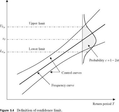
In practice, there are two ways to express the degree of uncertainty of a statistical quantity, namely, standard error and confidence interval (confidence limit). Because the estimated geophysical quantities of a particular return period are subject to uncertainty, they can be treated as a random variable associated with a distribution, as shown in Fig. 3.4. Similar to the standard deviation of a
|
random variable, the standard error of estimate se measures the standard deviation of an estimated statistical quantity from a sample, such as XT, about the true but unknown event magnitude. On the other hand, the confidence limit of an estimated quantity is an interval that has a specified probability (or confidence) to include the true value.
In the context of frequency analysis, the standard error of XT is a function of the distribution of the data series under consideration and the method of determining the distribution parameters. For example, the asymptotic (that is, as n ^ <x>) standard error of a T-year event se(XT) from a normal distribution can be calculated as (Kite, 1988)
f 2 + zT V/2
se (Xt ) = 2nT sx (3.21)
in which zT is the standard normal variate corresponding to the exceedance probability of 1/T, that is, Ф^т) = 1 – 1/T, n is the sample size, and sx is the sample standard deviation of random variable X. From the Gumbel distribution, the standard error of XT is
![]()
![]() Г 1 1 1/2
Г 1 1 1/2
1 + 1.1396 Kt + 1.1 KT sx
n
To construct the confidence interval for XT or for the frequency curve, a confidence level c that specifies the desired probability that the specified range will include the unknown true value is predetermined by the engineer. In practice, a confidence level of 95 or 90 percent is used. Corresponding to the confidence level c, the significance level a is defined as a = 1 – c; for example, if the desired confidence level c = 90 percent, the corresponding significance level a = 10 percent. In determining the confidence interval, the common practice is to distribute the significance level a equally on both ends of the distribution describing the uncertainty feature of estimated xT (see Fig. 3.4). In doing so, the boundaries of the confidence interval, called confidence limits, are defined. Assuming normality for the asymptotic sample distribution for XT, the approximated 100(1 – a) percent confidence interval for XT is
XT, a = XT – Z1-a/2 X Se(Xt) Xy, a = Xt + Z1-a/2 X Se(Xt) (3.23)
in which XT, a and XU, a are, respectively, the values defining the lower and upper bounds for the 100(1 – a) percent confidence interval, and z1-a/2 = Ф-1 (1 – a/2). The confidence interval defined by Eq. (3.23) is only approximate and the approximation accuracy increases with sample size.
Similar to the frequency-factor method, the formulas to compute the upper and lower limits of confidence interval for XT has the same form as Eq. (3.6), except that the frequency-factor term is adjusted as
XT, a = X + KTl a X Sx X%a = X + K% a X Sx (3.24)
in which K^ a and KU, a are the confidence-limit factors for the lower and upper limits of the 100(1 – a) percent confidence interval, respectively. For random samples from a normal distribution, the exact confidence-limit factors can be determined using the noncentral-t variates Z (Table 3.5). An approximation for K! p a with reasonable accuracy for n > 15 and a = 1 – c > 5 percent (Chowdhury et al., 1991) is
To compute KU, a, by symmetry, one only has to change za/2 by z1-a/2 inEq. (3.25). As was the case for Eq. (3.20), the confidence intervals defined by Eqs. (3.24) and (3.25) are most appropriate for samples from populations following a normal distribution, and for nonnormal populations, these confidence limits are only approximate, with the approximation accuracy increasing with sample size.
For Pearson type 3 distributions, the values of confidence-limit factors for different return periods and confidence levels given in Eq. (3.24) can be modified by introducing the scaling factor obtained from a first-order asymptotic
![]()
TABLE 3.5 95 Percent Confidence-Limit Factors for Normal Distribution
Return period (years)
|
n 2 5 10 25 50 100
|
approximation of the Pearson type 3 to normal quantile variance ratio n as (Stedinger et al., 1983)
Kr, a = Kt + n(ZT,1-a/2 — Zt ) and Ky, a = Kt + n(ZT, a/2 — Zt ) (3.26)
where
in which yx is the estimated skewness coefficient, and
A simulation study by Whitley and Hromadka (1997) showed that the approximated formula for the Pearson type 3 distribution is relatively crude and that a better expression could be derived for more accurate confidence-interval determination.
Example 3.8 Referring to Example 3.3, determine the 95 percent confidence interval of the 100-year flood assuming that the sample data are from a lognormal distribution.
Solution In this case, with the 95 percent confidence interval c = 0.95, the corresponding significance level a = 0.05. Hence Z0.025 = Ф—1(0.025) = —1.960 and г0.975 = Ф—1(0.975) = +1.960. Computation of the 95 percent confidence interval associated with the selected return periods are shown in the table below. Column (4) lists the values ofthe upper tail ofthe standard normal quantiles associated with each return period, that is, Kt = zt = Ф—1(1 — 1/T). Since random floods are assumed to be lognormally distributed, columns (7) and (8) are factors computed by Eq. (3.25) for defining the lower and upper bounds of the 95 percent confidence interval of different quantiles in log-space, according to Eq. (3.24), as
yT,0.95 = y + ZT,0.025 x sy yU,0.95 = y + ZT ,0.975 x sy
In the original space, the 95 percent confidence interval can be obtained simply by taking exponentiation as
ЧТ,0.95 = exp (уТ,0.95) and 3r,0.95 = exp (УТ,0.95)
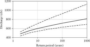
as shown in columns (11) and (12), respectively. The curves defining the 95 percent confidence interval, along with the estimated frequency curve, for a lognormal distribution are shown in Fig. 3.5.
|
95% CL for lognormal
Figure 3.5 95 percent confidence limits for a lognormal distribution applied to the annual maximum discharge for 19611975 on the Boneyard Creek at Urbana, IL. |
|
Exceedance |
Nonexceedance |
|||||
|
Return period |
probability |
probability |
||||
|
T (years) |
1 – p = 1/T |
p = 1 – 1/ T |
Kt = zt |
УТ |
qT |
|
|
(1) |
(2) |
(3) |
(4) |
(5) |
(6) |
|
|
2 |
0.5 |
0.5 |
0.0000 |
6.165 |
475.9 |
|
|
5 |
0.2 |
0.8 |
0.8416 |
6.311 |
550.3 |
|
|
10 |
0.1 |
0.9 |
1.2816 |
6.386 |
593.7 |
|
|
25 |
0.04 |
0.96 |
1.7505 |
6.467 |
643.8 |
|
|
50 |
0.02 |
0.98 |
2.0537 |
6.520 |
678.3 |
|
|
100 |
0.01 |
0.99 |
2.3263 |
6.567 |
711.0 |
|
|
Return period |
ZT,0.025 |
ZT,0.975 |
УТ,0.95 |
УТ,0.95 |
qT,0.95 |
qTU,0.95 |
|
T (years) |
(7) |
(8) |
(9) |
(10) |
(11) |
(12) |
|
2 |
– 0 . 54 |
0.54 |
6.071 |
6.259 |
433.2 |
522.8 |
|
5 |
0.32 |
1.63 |
6.221 |
6.446 |
503.1 |
630.4 |
|
10 |
0.71 |
2.26 |
6.288 |
6.555 |
538.1 |
702.9 |
|
25 |
1.10 |
2.96 |
6.355 |
6.676 |
575.5 |
792.8 |
|
50 |
1.34 |
3.42 |
6.397 |
6.755 |
600.1 |
858.2 |
|
100 |
1.56 |
3.83 |
6.434 |
6.827 |
622.8 |
922.2 |
In order to define confidence limits properly for the Pearson type 3 distribution, the skewness coefficient must be estimated accurately, thus allowing the frequency factor KT to be considered a constant and not a statistic. Unfortunately, with the Pearson type 3 distribution, no simple, explicit formula is available for the confidence limits. The Interagency Advisory Committee on Water Data (1982) (hereafter referred to as “the Committee”) proposed that the confidence limits for the log-Pearson type 3 distribution could be approximated using a noncentral ^-distribution. The committee’s procedure is similar to that of Eqs. (3.24) and (3.25), except that KT, a and KU a, the confidence-limit factors for the lower and upper limits, are computed with the frequency factor KT replacing ZT in Eq. (3.25).
Example 3.9 Referring to Example 3.3, determine the 95 percent confidence intervals for the 2-, 10-, 25-, 50-, and 100-year floods assuming that the sample data are from a log-Pearson type 3 distribution.
Solution From Example 3.3, the mean and standard deviation of the logarithms of the peak flows were 6.17 and 0.173, and the number of data n is 15. For the 100-year flood, Kt is 1.8164, and for the 95 percent confidence limits, a is 0.05; thus Za/2 is -1.96. Thus KT a is -0.651, and the lower 95 percent confidence bound is 427.2 ft3/s. The upper and lower confidence bounds for all the desired flows are listed in the following table:
|
Return Period T (years) |
Kt Eq. (3.8) |
KT,0.025 Eq. (3.26) |
KT,0.975 Eq. (3.26) |
qT,0.95 (ft3/s) |
au 4t,0.95 (ft3/s) |
|
2 |
-0.0907 |
-0.6513 |
0.4411 |
427.2 |
516.1 |
|
10 |
1.0683 |
0.5260 |
1.9503 |
523.7 |
670.1 |
|
25 |
1.4248 |
0.8322 |
2.4705 |
552.2 |
733.2 |
|
50 |
1.6371 |
1.0082 |
2.7867 |
569.3 |
774.4 |
|
100 |
1.8164 |
1.1540 |
3.0565 |
583.8 |
811.4 |


Leave a reply