Time-dependent reliability models for hydrosystems
Considering only inherent hydrologic uncertainty. Traditionally, the risk associated with the natural hydrologic randomness of flow or rainfall is explicitly considered in terms of a return period. By setting the resistance equal to the load with a return period of T years (that is, r* = lT), the annual reliability, without considering the uncertainty associated with lT, is 1 – 1/T, that is,
P (L < r *|r * = tT) = 1 – 1/T. Correspondingly, the reliability that the random loads would not exceed r * = lT in a period of t years can be calculated as (Yen, 1970)
Ps(t, T) = (4.108)
For large T, Eq. (4.108) reduces to
Ps(t, T) = exp( t/T) (4.109)
If T > t, Eq. (4.108) can further be approximated simply as ps(t, T) = 1 -1/T.
Considering both inherent hydrologic uncertainty and hydraulic uncertainty. In the
case where the uncertainty of the resistance is not negligible and is to be considered, the annual reliability of a hydrosystem infrastructure then has to be evaluated through load-resistance interference on an annual basis. That is, the annual reliability will be calculated by evaluating P(L < R) as Eq. (4.1), with f L(t) being the probability distribution function of annual maximum load. Hence the reliability of a hydrosystem over a service period of t years can be calculated by replacing the term 1/T in Eqs. (4.108) and (4.109) by 1 – P(L < R). Then the results are
Ps(t, L, R) = [P(L < R)]t (4.110)
Ps(t, L, R) = exp{—t x [1 – P(L < R)]} (4.111)
in which the evaluation of annual reliability P (L < R) can be made through the reliability methods described in preceding sections.
Incorporation of a design event. In the design of hydraulic structures, the common practice is to determine the design capacity based on a preselected design return period tT and safety factor SF. Under such a condition, the magnitude of the future annual maximum hydrologic load can be partitioned into two complementary subsets, that is, t < tT and t > tT, with each representing different recurrence intervals of the hydrologic process. The reliability of the hydrosystem subject to the ith hydrologic load occurring in the future can be expressed by using the total probability theorem (Sec. 2.2.4) as
Ps, i = P (Li < r)
= P(Li < r |Li > tT) P(Li > tT) + P(Li < r |Li < tT) P (Li < tT)
= P (tT < Li < r) + P (Li < r, Li < tT)
= P1 + P 2 (4.112)
where Pi and P2 can be written explicitly as
 |
![]()
 |
r
 |
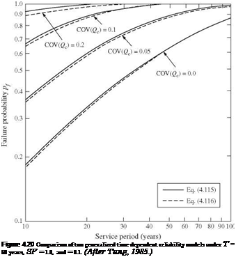
probability computed by the two models converge as the service life increases. Without considering hydraulic uncertainty [i. e., Cov(Qc) = 0], the failure probability is significantly underestimated. Computationally, the time-dependent model based on the binomial distribution, i. e., Eq. (4.39a), is much simpler than that based on the Poisson distribution.


Leave a reply