Stratified sampling technique
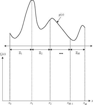
The stratified sampling technique is a well-established area in statistical sampling (Cochran, 1966). Variance reduction by the stratified sampling technique is achieved by taking more samples in important subregions. Consider a problem in which the expectation of a function g (X) is sought, where X is a random variable with a PDF fx(x), x є E. Referring to Fig. 6.13, the domain E for the random variable X is divided into M disjoint subregions Em, m = 1, 2,…, M. That is,
m
S = U Sm 0 = Sm Fl Sm! m = m
m=1
|
|
Let pm be the probability that random variable X will fall within the subregion Em, that is, f fx(x)dx = pm. Therefore, it is true that Lmpm = 1.
The expectation of g (X) can be computed as
m.. M
G = g(x) fx(x) dx =^2 / g(x) fx(x) dx =^2 Gm (6.86)
m=1J Em m=1
where Gm = fw g (x) fx(x) dx.
Note that the integral for Gm can be written as
 |
|
|
|
|
|
|

 |
|||
where nm is the number of sample points in the mth subregion, and Lmnm = n, the total number of random variates to be generated. Therefore, the estimator for G in Eq. (6.86) can be obtained as
After the number of subregions M and the total number of samples n are determined, an interesting issue for the stratified sampling is how to allocate the total n sample points among the M subregions such that the variance associated with G by Eq. (6.89) is minimized. A theorem shows that the optimal n*m that minimizes Var(G) in Eq. (6.89) is (Rubinstein, 1981)
![]()
 pm&m
pm&m
v^M p _
Xm’ = 1 P m’ °m!
where am is the standard deviation associated with the estimator Gm in Eq. (6.88).
In general, information about am is not available in advance. It is suggested that a pilot simulation study be made to obtain a rough estimation about the value of am, which serves as the basis in the follow-up simulation investigation to achieve the variance-reduction objective.
A simple plan for sample allocation is nm = npm after the subregions are specified. It can be shown that with this sampling plan, the variance associated with G by Eq. (6.89) is less than that from the simple random-sample technique. One efficient stratified sampling technique is systematic sampling (McGrath, 1970), in which pm = 1/M and nm = n/M. The algorithm of the systematic sampling can be described as follows:
1. Divide interval [0, 1] into M equal subintervals.
2. Within each subinterval, generate n/M uniform random numbers umi ~ U[(m — 1)/n, m/n], m = 1, 2,…, M; i = 1, 2,…, n/m.
3. Compute Xmi = F—l(Umi).
4. Calculate G according to Eq. (6.89).
Example 6.13 Referring to Example 6.7, apply the systematic sampling technique to evaluate the pump failure probability in the time interval [0, 200 h].
Solution Again, let us adopt the uniform distribution U(0, 200) and carry out the computation by the sample-mean Monte Carlo method. In the systematic sampling, the interval [0, 200] is divided into 10 equal-probability subintervals, each having a probability content of 0.1. Since h(t) = 1/200, 0 < t < 200, the end points of each subinterval can be obtained easily as
tQ = 0, t1 = 20, t2 = 40,…, t9 = 180, t10 = 200
Furthermore, let us generate nm = 200 random variates from each subinterval so that £mnm = 2000. This can be achieved by letting
|
|||
|
|
||
|
|||
The algorithm for estimating the pump failure probability is the following:
1. Initialize subinterval index m = 0.
2. Let m = m + 1. Generate nm = 200 standard uniform random variates {um1, um2,…, um,200}, and transform them into the random variates from the corresponding subinterval by tmi = 20(m — 1) + 20umi, for i = 1, 2,…, 200.
3. Compute pf, m as
pf, m = 200 5-/ ft(tmi)
mi = 1
and the associated variance as
![]() p2 s2 0 12s2
p2 s2 0 12s2
m m. m
nm 200
in which sm is the standard deviation of 200 ft(tmi) for the mth subinterval.
4. If m < 10, go to step 2; otherwise, compute the pump failure probability as
1 10
P f = 10 E p f m
m=1
and the associated standard error as
|
|
|
|
|
|
m=1
|
The results from the numerical simulation are shown below:
The value of pf is extremely close to the exact solution of 0.147856. |


Leave a reply