Reliability design with redundancy

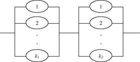
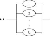
Consider the design of a hydrosystem consisting of n subsystems that are ar­ranged in series so that the failure of one subsystem will cause the failure of the entire system. In this case, reliability of the hydrosystem can be improved by installing standby units in each subsystem (see Fig. 8.7). Figure 8.7 consists of a series-parallel configuration that is called unit redundancy. Suppose that each subsystem can install up to K standby units and that the total capital available for the hydrosystem is C. Furthermore, the cost functions are known, with Ci (ki) being the cost associated with installing ki standby units on the ith subsystem.

Suppose that the engineer is interested in determining the number ofstandby units for each subsystem to maximize the system reliability asys without

Subsystem 1	Subsystem 2	Subsystem n
Figure 8.7 Unit redundancy with series-parallel configuration.

exceeding the available capital. The optimization model for the problem can be expressed as

n

Maximize asys = ]^[ at (ki) (8.11a)

i = 1 n

subject to ‘^JCi(kt) < C (8.11b)

i=1

where kt is the nonnegative integer-valued decision variable, 0 < kt < K, and at (ki) is the reliability of the ith subsystem installed with kt standby units.

This optimization problem can be solved efficiently by the DP approach de­scribed in Sec. 8.1.3. The stages are the subsystems i = 1, 2,…, n. The DP backward-recursive equation can be written as

max[ai (ki)] i = n

ki

max{ai(ki) x f i+1 [b; — Ci(ki)]} i = 1, 2,…, n — 1

ki where bi is the state variable representing the total capital available for subsystems i, i + 1,…, n.

Alternatively, the design engineer may be interested in finding the system configuration associated with the least total capital investment while achieving some acceptable reliability for the system asys, min. The problem of this type can be expressed by the following model:

n

Minimize ‘^2/Ci (ki) (8.13a)

i=1

n

subject to ]^[ ai(ki) ^ asys, min (8.13b)

i=1

The model defined by Eqs. (8.13a-b) also can be solved by the DP approach. To illustrate the application of other optimization procedure, let the reliability
of each standby unit in each subsystem be equal to at and the unit cost be Ci, i = 1, 2,, n. Furthermore, the minimum acceptable system reliability is set equal to asys, min. Then, Eqs. (8.13a-b) can be rewritten as

n

Minimize Y. ciki (8.14a)

i=1

n

subject to [1 — (1 — ai)ki] = aSyS, min (8.14b)

i=1

The model, Eqs. (8.14a-b), involves a linear objective function and a nonlinear equality constraint. To simplify the multiplicative relationship of Eq. (8.14b), a new variable pi is defined to satisfy the following equation:

In terms of the new variable pi, the original decision variable ki and the con­straint Eq. (8.14b) can be expressed, respectively, as

Therefore, the original model, Eqs. (8.14 a-b), can be written as

This constrained minimization problem, Eqs. (8.16a-b), can be solved by mini­mizing the following Lagrangian function:

(8.17)

Solving

Ci d (! — asPys, min) (1 — asys, mi^(1 — ai) dPi + A = 0 i = 1, 2,…, n

d L( P1, P2, …, Pn, A)

d Pi

(8.18)

results in

c aPi ln! aPi і

к i asys, min Vasys, min/

(! — asys, min)(1 — ai)

Suppose that the minimum acceptable system reliability asys, min is chosen to be close to 1. In such a case,

which renders

Then, by Eqs. (8.22) and (8.23), the new variable pi can be obtained, in terms of the unit cost ci, and reliability of standby unit ai, as

(8.24)

Once the values of pi’s are computed by Eq. (8.24), the number of standby units for each subsystem ki can be obtained by Eq. (8.15a). Finally, one should realize that the values of ki so obtained are not guaranteed to be integer-valued. A round-off to the closest integer may be needed.