Probability Estimates for Data Series: Plotting Positions (Rank-order Probability)
As stated previously, the objective of frequency analysis is to fit geophysical data to a probability distribution so that a relationship between the event magnitude and its exceedance probability can be established. The first step in the procedure is to determine the type of data series (i. e., event magnitude) to be used. In order to fit a probability distribution to the data series, estimates of probability (or equivalent return period) must be assigned to each magnitude in the data series.
Consider a data series consisting of the entire population of N values for a particular variable. If this series were ranked according to decreasing magnitude, it could be stated that the probability of the largest variate being equaled or exceeded is 1/N, where N is the total number of variates. Similarly, the exceedance probability of the second largest variate is 2/N, and so forth. In general,
1 m
P(X > X(m)) = — = – (3.2)
in which m is the rank of the data in descending order, x—) is the mth largest variate in a data series of size N, and Tm is the return period associated with x—). In practice, the entire population is not used or available. However, the reasoning leading to Eq. (3.2) is still valid, except that the result is now only an estimate of the exceedance probability based on a sample. Equation (3.2), which shows the ranked-order probability, is called a plotting position formula because it provides an estimate of probability so that the data series can be plotted (magnitudes versus probability).
Equation (3.2) is appropriate for data series from the population. Some modifications are made to avoid theoretical inconsistency when it is applied to sample data series. For example, Eq. (3.2) yields an exceedance probability of 1.0 for the smallest variate, implying that all values must be equal or larger. Since only
a sample is used, there is a likelihood that at some future time an event with a lower value could occur. In application, if the lower values in the series are not of great interest, this weakness can be overlooked, and in fact, Eq. (3.2) is used in the analysis of the annual exceedance series. A number of plotting-position formulas have been introduced that can be expressed in a general form as
1 m — a
P(x > x(m)) = um = — = n + 1 _ b (3.[1]
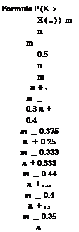
in which a > 0 and b > 0 are constants, and n is the number of observations in the sample data series. Table 3.2 lists several plotting-position formulas that have been developed and used in frequency analysis. Perhaps the most popular plotting-position formula is the Weibull formula (with a = 0 and b = 0):
1 m
P{X > X(m)) = Um = ^ = ^^ (3.4)
Tm n + 1
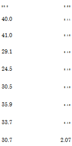
As shown in Table 3.2, it is noted that although these formulas give different results for the highest values in the series, they yield very similar results for the middle to lowest values, as seen in the last two columns.
Plotting-position formulas in the form of Eq. (3.3) can be categorized into being probability-unbiased and quantile-unbiased. The probability-unbiased
![]()
![]()

 |
 |
TABLE 3.2 Plotting-Position Formulas
plotting-position formula is concerned with finding a probability estimate u(m) for the exceedance probability of the mth largest observation such that E[G(X(m))] = u(m), in which G(X(m>) = P(X > X(m>). In other words, the probability-unbiased plotting position yields the average exceedance probability for the mth largest observation in a sample of size n. If the data are independent random samples regardless of the underlying distribution, the estimator U(m) = G(X (m)) will have a beta distribution with the mean E (U(m)) = m/(n+l). Hence the Weibull plotting-position formula is probability-unbiased. On the other hand, Cunnane (1978) proposed quantile-unbiased plotting positions such that average value of the mth largest observation should be equal to G-1(u(m>), that is, E(X(m)) = G-1(u(m)). The quantile-unbiased plotting-position formula, however, depends on the assumed distribution G( ). For example, referring to Table 3.2, the Blom plotting-position formula gives nearly unbiased quantiles for the normal distribution, and the Gringorton formula gives nearly unbiased quantiles for the Gumbel distribution. Cunnane’s formula, however, produces nearly quantile-unbiased plotting positions for a range of distributions.


Leave a reply