Orthogonal Transformation Techniques

The orthogonal transformation is an important tool for treating problems with correlated stochastic basic variables. The main objective of the transformation is to map correlated stochastic basic variables from their original space to a new domain in which they become uncorrelated. Hence the analysis is greatly simplified.

Consider K multivariate stochastic basic variables X = (Xі, X2,, XK)t having a mean vector fj, x = (jx1, /г2 …, /гкУ and covariance matrix Cx as
011 012 013 021 °22 023
01K 02K
Cr =
0K1 Ok2 0K3	okk
in which oij = Cov(Xi, Xj), the covariance between stochastic basic variables Xi and Xj. The vector of correlated standardized stochastic basic variables X’ = D-1/2(X — fxx), that is, X’ = (X1, X2,…, XKУ with Xk = (Xk — /xk)/ok, for k = 1,2,…, K, and Dx being an K x K diagonal matrix of variances of stochastic basic variables, that is, D x = diag(o12, o|, …, o^), would have a mean vector of 0 and the covariance matrix equal to the correlation matrix Rx:
Y = T-1X ’ (4C.1) where Y is a vector with the mean vector 0 and covariance matrix I, a K x K identity matrix. Stochastic variables Y are uncorrelated because the off- diagonal elements of the covariance matrix are all zeros. If the original stochas­tic basic variables X are multivariate normal variables, then Y is a vector of uncorrelated standardized normal variables specifically designated as Z’ be­cause the right-hand side of Eq. (4C.1) is a linear transformation of the normal random vector. It can be shown that from Eq. (4C.1), the transformation matrix T must satisfy
Rx = TTt
(4C.2)

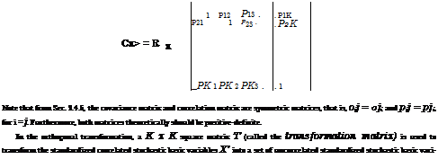
There are several methods that allow one to determine the transformation matrix in Eq. (4C.2). Owing to the fact that Rx is a symmetric and positive — definite matrix, it can be decomposed into

Rx = LLt (4C.3)

in which L is a K x K lower triangular matrix (Young and Gregory, 1973; Golub and Van Loan, 1989):

l11 0	0	. . . 0 ‘
l21 l22	0	. . . 0
Ik 1 Ik2 Ik3	. . . Ikk _

L

which is unique. Comparing Eqs.(4C.2) and (4C.3), the transformation matrix T is the lower triangular matrix L. An efficient algorithm to obtain such a lower triangular matrix for a symmetric and positive-definite matrix is the Cholesky decomposition (or Cholesky factorization) method (see Appendix 4B).

The orthogonal transformation alternatively can be made using the eigenvalue-eigenvector decomposition or spectral decomposition by which Rx is decomposed as

Rx = Cx = VAVt (4C.4)

where V is a K x K eigenvector matrix consisting of K eigenvectors as V = (v i, v 2,…, vK), with vk being the kth eigenvector of the correlation matrix Rx, and Л = diag(X1, Л2,…, XK) being a diagonal eigenvalues matrix. Frequently, the eigenvectors v’s are normalized such that the norm is equal to unity, that is, vt v = 1. Furthermore, it also should be noted that the eigenvectors are or­thogonal, that is, v t v j = 0, for i = j, and therefore, the eigenvector matrix V obtained from Eq. (4C.4) is an orthogonal matrix satisfying VVt = Vt V = I where I is an identity matrix (Graybill, 1983). The preceding orthogonal trans­form satisfies

Vt Rx V = Л (4C.5)

To achieve the objective of breaking the correlation among the standardized stochastic basic variables X’, the following transformation based on the eigen­vector matrix can be made:

U = VtX’ (4C.6)

The resulting transformed stochastic variables U has the mean and covariance matrix as

E(U) = V tE(X’) = 0 C (U) = VtCx V = Vt RxV = Л

(4C.7a) (4C.7b)

and

As can be seen, the new vector of stochastic basic variables U obtained by Eq. (4C.6) is uncorrelated because its covariance matrix Cu is a diagonal ma­trix Л. Hence, each new stochastic basic variable Uk has the standard deviation equal to V^k, for all k = 1, 2,…, K.

The vector U can be standardized further as

Y = Л-1/2и (4C.8)

Based on the definitions of the stochastic basic variable vectors X — (vx, Cx), X’ — (0, Rx), U — (0, Л), and Y — (0,1) given earlier, relationships between them can be summarized as the following:

Y = Л-1/2и = Л-1/2 V1X’ (4C.9)

Comparing Eqs.(4C.1) and (4C.9), it is clear that

T-1 = Л-1/2 V1

Applying an inverse operator on both sides of the equality sign, the transfor­mation matrix T alternatively, as opposed to Eq. (4C.3), can be obtained as

T = VЛ1/2 (4C.10)

Using the transformation matrix T as given above, Eq. (4C.1) can be expressed as

X ‘ = TY = VЛ1/2Y (4C.11a)

and the random vector in the original parameter space is

X = vx + D1/2 VЛ1/2Y = vx + D1/2 LY (4C.11b)

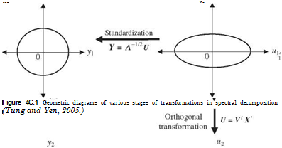
Geometrically, the stages involved in orthogonal transformation from the orig­inally correlated parameter space to the standardized uncorrelated parameter space are shown in Fig. 4C.1 for a two-dimensional case.

From Eq. (4C.1), the transformed variables are linear combinations of the standardized original stochastic basic variables. Therefore, if all the original stochastic basic variables X are normally distributed, then the transformed stochastic basic variables, by the reproductive property of the normal random variable described in Sec. 2.6.1, are also independent normal variables. More specifically,

X — N(vx, Cx) X’ — N(0, Rx) U — N(0, Л) and Y = Z — N(0,1)

The advantage of the orthogonal transformation is to transform the correlated stochastic basic variables into uncorrelated ones so that the analysis can be made easier.

The orthogonal transformations described earlier are applied to the stan­dardized parameter space in which the lower triangular matrix and eigenvector matrix of the correlation matrix are computed. In fact, the orthogonal transfor­mation can be applied directly to the variance-covariance matrix Cx. The lower triangular matrix of Cx, L, can be obtained from that of the correlation matrix L by

L = D1/2 L (4C.12)

Following a similar procedure to that described for spectral decomposition, the uncorrelated standardized random vector Y can be obtained as

Y = Л-1/2 Vг (X — цх) = Л-1/2£7 (4C.13)

where V and Л are the eigenvector matrix and diagonal eigenvalue matrix of the covariance matrix Cx satisfying

Cx = УЛ V/1

and U is an uncorrelated vector of the random variables in the eigenspace having a zero mean 0 and covariance matrix Л. Then the original random vector X can be expressed in terms of Y and L:

X = fix + VA1/2Y = fix + L Y (4C.14)

One should be aware that the eigenvectors and eigenvalues associated with the covariance matrix Cx will not be identical to those of the correlation matrix Rx.