Graphic Approach

Once the data series is identified and ranked and the plotting position is calcu­lated, a graph of magnitude x versus probability [P(X > x), P(X < x), or T] can be plotted and a distribution fitted graphically. To facilitate this procedure, it is common to use some specially designed probability graph paper rather than linear graph paper. The probability scale in those special papers is chosen such that the resulting probability plot is a straight line. By plotting the data using a particular probability scale and constructing a best-fit straight line through the data, a graphic fit is made to the distribution used in constructing the prob­ability scale. This is a graphic approach to estimate the statistical parameters of the distribution.

Example 3.1 illustrates the graphic approach to the analysis of flood data. The general procedure is as follows: [2] [3] 3 [4]

5. Extend the line to the highest return-period value needed, and read all re­quired return-period values off the line.

Example 3.1 The Boneyard Creek stream gauging station was located near the fire station on the campus of the University of Illinois at Urbana-Champaign. From the USGS Water Supply Papers, the partial duration data of peak discharges above 400 ft3/s between the water years 1961 and 1975 were obtained and listed below. In addi­tion, for the years when there was no flow in a year exceeding 400 ft3/s, the peak flow for that year is given in parenthesis (e. g., 1961).

(a) List the ranked annual maximum series. Also compute and list the corresponding plotting positions (return period) and exceedance probability P (X > x).

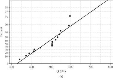
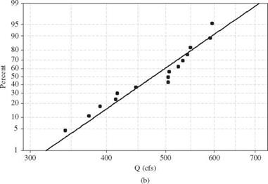
(b) Plot the annual maximum series on (i) Gumbel paper and (ii) lognormal paper.

(c) Construct a best-fit line through the nonlinear plots, and estimate the flows for return periods of 2, 10, 25, and 50 years.

Solution n = 15 (a)

(b) Plots of the annual maximum flow series on the Gumbel and lognormal probability papers are shown in Fig. 3.2.