Gram-Schmid Ortho-normalization

Consider a vector x 1 in an K-dimensional space to be used as one of the basis vectors. It is desirable to find the additional vectors, along with x 1, so that they would form K orthonormal basis vectors for the K-dimensional space. To do that, one can arbitrarily select K — 1 vectors in the K-dimensional space as x 2, x3, …, xK.

The first basis vector can be obtained as u1 = x 1/|x1|. Referring to Fig. 4D.1, a second basis vector (not necessarily normalized) that will be orthogonal to the first basis vector u1 can be derived as

У 2 = x2 — У2 = x2 — (x2«0«1

Therefore, the second normalized basis vector u2, that is perpendicular to u2 can be determined as u2 = y2/|y2|.

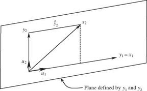
Note that the third basis vector must be orthogonal to the previously deter­mined basis vectors (u1, u2) or (y 1, y 2). Referring to Fig. 4D.2, the projection of x 3 onto the plane defined by y1 and y 2 is

Уз = (x 3u1) u1 + (x 3u2) u2

Figure 4D.1 Determination of the second basis vector.

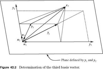
Therefore, the third basis vector У3 that is orthogonal to both y1 and y2 can be determined as

Уз = xз — Уз = xз — [(x“1 + (x3^)“2]

and the corresponding normalized basis vector u3 can be determined as u3 = У3/ІУ3І-

From the preceding derivation, the kth basis vector yk can be computed as

In the case that x2, x3,…, xK are unit vectors, the basis vectors У2, У3,…, УК obtained by Eq. (4D.1) are orthonormal vectors. It should be noted that the results Gram-Schmid orthogonalization is dependent on the order of vectors x2,x3,…,xK selected in the computation. Therefore, the orthonormal basis from the Gram-Schmid method is not unique.

The preceding Gram-Schmid method has poor numerical properties in that there is a severe loss of orthogonality among the generated yk (Golub and Van Loan, 1989). The modified Gram-Schmid algorithm has the following steps:

1. k = 0.

2. Let k = k + 1 and yk = xk, for k = 1. Normalize vector yk as uk = yk/|yk |.

3. For k + 1 < j < К, compute the vector of xj projected on uk:

У] = (x j uk)uk and the component of xj orthogonal to ui as

У j = xj — yj = xj — (xj — uk) uk

4. Go to step 2 until k = К.

4.1 Refer to Sec. 1.6 for the central safety factor. Assuming that both R and L are independent normal random variables, show that the reliability index в is related to the central safety factor as

MSF — 1

mSf QR + QL

in which Qx represents the coefficient of variation of random variable X.

4.2 Referring to Problem 4.1, the central safety factor can be expressed in terms of reliability index в as

1 + в Qr + Q — в2qR QL 1 — e2oR

4.3 Referring to Problem 4.1, how should the equation be modified if the resistance and load are correlated?

4.4

Refer to Sec. 1.6 for the characteristic safety factor. Let Ro be defined on the lower side of resistance distribution as Ro = rp with P(R < rp) = p (see Fig. 4P.1). Similarly, let Lo be defined on the upper side of load distribution with Lo = t1-q. Consider that R and L are independent normal random variables. Show that characteristic safety factor SFc is related to the central safety factor as

in which Zp = Ф 1(p).

4.5 Define the characteristic safety factor as the ratio of the median resistance to the median load as

SF = Г05 = Г

^0.5 t

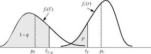
where Г = r0.5 = F_-1(0.5)and t = to.5 = F_-1(0.5), with Fr(■) and Fl(-) being the CDFs of the resistance and load, respectively. Suppose that the resistance R

and load L are independent lognormal random variables. Show that the central safety factor hsf = HR/HL is related to SF as

1 + QR 1 + Q

4.6

Referring to Problem 4.4, show that for independent lognormal resistance and load, the following relation holds:

Let W(X) = X1 + X2 — c, in which X1 and X2 are independent stochastic vari­ables with PDFs, f 1(x1) and f 2(X2), respectively. Show that the reliability can be computed as

/* TO

f 1(X1)[1 — F2(c — X1)]dx1

f 2(X2)[1 — F1(c — X2)]dX2

4.7 Suppose that the load and resistance are independent random variables and that each has an exponential PDF as

fX(x) = XX exp(— Xxx) for X > 0

in which x can be the resistance R and load L. Show that the reliability is

bL HR

Ps = 1—T1— = —г—

Xl + Xr hr + HL

Show that the reliability for independently normally distributed resistance (with mean hr and standard deviation or ) and exponentially distributed load (with the mean 1/Xl) is

4.10 Suppose that the annual maximum flood in a given river reach has Gumbel dis­tribution [Eq. (2.85a)] with mean hl and coefficient of variation Ql. Let the levee system be designed to have the mean capacity of hR = SFc x It, with SFc being the characteristic safety factor and T-year flow, respectively. For simplic­ity, assume that the levee conveyance capacity has a symmetric PDF, as shown in Fig. 4P.2. Derive the expression for the levee reliability assuming that flood magnitude and levee capacity are independent random variables.

4.11 Numerically solve Problem 4.10 using the following data:

HL = 6000 ft3/s Ql = 0.5 T = 100 years a = 0.15

for SFc = 1.0 and 1.5.

fr (r)

	О ON
	0.2	0.2	————- ►

(l — a)Vr Vr (i + a)m Figure 4P.2

4.12 Consider that load and resistance are independent uniform random variables with PDFs as

Load: fb(0 = 1/(^ — Р ^ < I < ^

Resistance: fR (r) = 1/(r2 — r 1) r 1 < r < Г2

Furthermore, I1 < r 1 < I2 < r2, as shown in Fig. 4P.3. Derive the expression for the failure probability.

4.13 Consider that load and resistance are independent random variables. The load has an extreme type I (max) distribution [Eq. (2.85a)], with the mean 1.0 and standard deviation of 0.3, whereas the resistance has a Weibull distribution [Eq. (2.89)], with mean 1.5 and standard deviation 0.5. Compute the failure prob­ability using appropriate numerical integration technique.

4.14 Consider that the annual maximum flood has an extreme type I (max) distribu­tion with the mean 1000 m3/s and coefficient of 0.3. On the other hand, the levee capacity has a lognormal distribution with a mean of 1500 m3/s and coefficient of variation of 0.2. Assume that flood and levee capacity are two independent random variables. Compute the failure probability that the levee will be over­topped using appropriate numerical integration technique.

4.15 Resolve Example 4.6 taking into account the fact that stochastic variables n and D are correlated with a correlation coefficient —0.75.

		fR(r)7
	1 1 1 1 1 _______________ 1_____	1 1 1 1 1

fd-O

z

ri Є

€1

4.16 The annual benefit and cost of a small hydropower project are random variables, and each has a Weibull distribution [see Eq. (2.89)] with the following distribu­tional parameter values:

	a	$	в
Benefit	4.5422	60,000	266,000
Cost	3.7138	100,000	110,000

(a) Compute the mean and standard deviation of the annual benefit and cost.

(b) Assume that the annual benefit and cost are statistically independent. Find out the probability that the project is economically feasible, i. e., the annual benefit exceeds the annual cost.

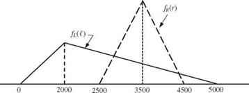
4.17 Suppose that at a given dam site the flood flows and the spillway capacity follow triangular distributions, as shown in Fig. 4P.4. Use the direct integration method to calculate the reliability of the spillway to convey the flood flow (Mays and Tung, 1992).

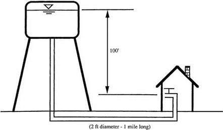
The Hazen-Williams equation is used commonly to compute the head losses in a water distribution system, and it is written as

€ , r

Figure 4P.5 (After Mays and Tung, 1992).

the uncertainty in pipe roughness and pipe diameter, the supply to the user is not certain. We know that the pipe has been installed for about 3 years. Therefore, our estimation of the pipe roughness in the Hazen-Williams equation is about 130 with some error of ±20. Furthermore, knowing the manufacturing tolerance, the 1-ft pipe has an error of ±0.05 ft. Assume that both the pipe diameter and Hazen — Williams’ Chw coefficient have lognormal distributions with means of 1 ft and 130 and standard deviations of 0.05 ft and 20, respectively. Using the MFOSM method, determine the reliability that the demand of the user can be satisfied (Mays and Tung, 1992).

4.19 In the design of storm sewer systems, the rational formula

Ql = CiA

is used frequently, in which Ql is the surface inflow resulting from a rainfall event of intensity i falling on the contributing drainage area of A, and C is the runoff coefficient. On the other hand, Manning’s formula for full pipe flow, that is,

Qc = 0.463n-1 S1/2 D8/3

is used commonly to compute the flow-carrying capacity of storm sewers, in which D is the pipe diameter, n is the Manning’s roughness, and S is pipe slope.

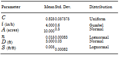
Consider that all the parameters in the rational formula and Manning’s equa­tion are independent random variables with their mean and standard deviation given below. Compute the reliability of a 36-in pipe using the MFOSM method (Mays and Tung, 1992).

In most locations, the point rainfall intensity can be expressed by the following empirical rainfall intensity-duration-frequency (IDF) formula:

. aTm

i = 1———

b + tc

where i is the rainfall intensity (in in/h or mm/h), t is the storm duration (in minutes), T is the return period (in years), and a, m, b, and c are constants.

At Urbana, Illinois, the data analysis results in the following information about the coefficients in the preceding rainfall IDF equation:

Variable	Mean, і	Coef. ofVar. ^	Distribution
a	120	0.10	Normal
b	27	0.10	Normal
c	1.00	0.05	Normal
m	0.175	0.08	Normal

Assuming independence among the IDF coefficients, analyze the uncertainty of the rainfall intensity for a 10-year, 24-minute storm. Furthermore, incorporate the derived information herein to Problem 4.19 to evaluate the sewer reliability.

The storm duration used in the IDF equation (see Problem 4.20) in general is equal to the time of concentration. One of the most commonly used in the Kirpich (Chow, 1964):

tc = C (^ У

where tc is the time of concentration (in minutes), L is the length of travel (in feet) from the most remote point on the drainage basin along the drainage channel to the basin outlet, S is the slope (in ft/ft) determined by the difference in elevation of the most remote point and that of the outlet divided by L, and c1 and c2 are coefficients.

Assume that c1 and c2 are the only random variables in the Kirpich formula with the following statistical features:

Parameter	Mean	Coeff. ofVar.	Distribution
c1	0.0078	0.3	Normal
c1	0.77	0.2	Normal

(a) Determine the mean and standard deviation of tc for the basin with L = 1080 ft and S = 0.001.

(b)

Incorporate the uncertainty feature of tc obtained in (a), and resolve the sewer reliability as Problem 4.20.

(c) Compare the computed reliability with those from Problems 4.19 and 4.20.

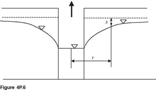
Referring to Fig. 4P.6, the drawdown of a confined aquifer table owing to pumping can be estimated by the well-known Copper-Jacob equation:

in which § is the model correction factor accounting for the error of approximation, s is the drawdown (in meters), S is the storage coefficient, T is the transmissiv­ity (in m2/day), Qp is the pumping rate (in m3/day), and t is the elapse time (in days). Owing to the nonhomogeneity of geologic formation, the storage coef­ficient and transmissivity are in fact random variables. Furthermore, the model correction factor can be treated as a random variable. Given the following in­formation about the stochastic variables in the Copper-Jacob equation, estimate the probability that the total drawdown will exceed 1.5 m under the condition of Qp = 1000 m3/day, r = 200 m, and t = 7 days by the MFOSM method.

Variable	Mean n	Coeff. ofVar.	Distribution
§	1.000	0.10	Normal
T (m2/day)	1000.0	0.15	Lognormal
S	0.0001	0.10	Lognormal

NOTE: p(T, S) = -0.70; p(§, T) = 0.0; p(§, S) = 0.0.

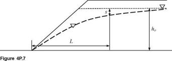
4.23 Referring to Fig. 4P.7, the time required for the original phreatic surface at ho to have a drawdown s at a distance L from the toe of a cut slope can be approximated by (Nguyen and Chowdhury, 1985)

s = 1 — erf =

ho 2 у/Khot /S

where erf(x) is the error function, which is related to the standard normal CDF as erf(x) = 2^/2[Ф(x) — 0.5], K is the conductivity of the aquifer, S is the storage coefficient, and t is the drawdown time. From the slope stability viewpoint, it is

required that further excavation can be made safely only when the drawdowns reach at least half the original phreatic head. Therefore, the drawdown time to reach sfho = 0.5 can be determined from the preceding equation as

*=(I)2 Kb

where § = erf 1(0.5) = 0.477.

Consider that K and S are random variables having the following statistical properties:

Variable	Mean і	Std. Dev. a	Distribution
K (m/day)	0.1	0.01	Lognormal
S	0.05	0.005	Lognormal
NOTE: p(K, S) = 0.5.

Estimate the probability by the MFOSM method that the drawdown time td will be less than 40 days under the condition L = 50 m and ho = 30 m.

4.24 The one-dimensional convective contaminant transport in steady flow through porous media can be expressed as (Ogata, 1970):

C(x, t) 1 x — (q/n)t

erfc

Co 2 2 V ai(q/n)t

in which C(x, t) is the concentration at point x and time t, Co is the concentration of the incoming solute, x is the location along a one-dimensional line, q is the specific discharge, n is the porosity, ai is the longitudinal dispersivity, erfc is the complimentary error function, erfc(x) = 1 — erf(x), and t is the time.

Assume that the specific discharge q, longitudinal dispersivity ai, and porosity n are random variables with the following statistical properties:

Variable	Mean і	Std. Dev. a	Distribution
q (m/day)	1.0	0.10	Lognormal
n	0.2	0.02	Normal
ai(m)	10.0	1.00	Lognormal

NOTE: p(n, ai) = 0.75; zero for other pairs.

Estimate P [C(x, t)/Co > 0.5] for x = 525 m and t = 100 days by the MFOSM method.

4.25

Referring to the following Streeter-Phelps equation:

consider that the deoxygenation coefficient Kd, the reaeration coefficient Ka, the average stream velocity U, the initial dissolved oxygen DO, deficit concentrations D0, and the initial in-stream BOD concentration L0 are random variables. As­suming a saturated DO concentration of 8.48 mg/L, use the MFOSM method to estimate the probability that the in-stream DO concentration will be less than 4.0 mg/L at x = 10 miles downstream of the waste discharge point by adopting a lognormal distribution for the DO concentration with the following statistical properties for the involved random variables:

Variable	Mean u	Std. Dev. a	Distribution
Kd	0.60 L/day	0.060 L/day	Lognormal
Ka	0.76 L/day	0.076 L/day	Lognormal
U	1.2 ft/sec	0.012 ft/sec	Normal
D0	1.60 mg/L	0.160 mg/L	Normal
L0	6.75 mg/L	0.0675 mg/L	Normal

NOTE: p(Ka, U) = 0.8 and zero for all other pairs.

4.26 Referring to the Steeter-Phelps equation in Problem 4.25, determine the criti­cal location associated with the maximum probability that the DO concentration is less than 4.0 mg/L using the statistical properties of involved random vari­ables given in Problem 4.25. At any trial location, use the MFOSM method, along with the lognormal distribution for the random DO concentration, to compute the probability.

4.27 Develop a computer program for the Hasofer-Lind algorithm that can be used for problems involving correlated nonnormal random variables.

4.28 Develop a computer program for the Ang-Tang algorithm that can be used for problems involving correlated nonnormal random variables.

4.29 Solve Problem 4.18 by the AFOSM method. Also compute the sensitivity of the failure probability with respect to the stochastic variables. Compare the results with those obtained in Problem 4.18.

4.30 Solve Problem 4.21 by the AFOSM method considering all stochastic basic vari­ables involved, and compare the results with those obtained in Problem 4.21.

4.31 Solve Problem 4.22 by the AFOSM method considering all stochastic basic vari­ables involved, and compare the results with those obtained in Problem 4.22.

4.32 Solve Problem 4.23 by the AFOSM method considering all stochastic basic vari­ables involved, and compare the results with those obtained in Problem 4.23.

4.33 Solve Problem 4.24 by the AFOSM method considering all stochastic basic vari­ables involved, and compare the results with those obtained in Problem 4.24.

4.34 Solve Problem 4.25 by the AFOSM method considering all stochastic basic vari­ables involved, and compare the results with those obtained in Problem 4.25.

4.35 Solve Problem 4.26 by the AFOSM method considering all stochastic basic vari­ables involved, and compare the results with those obtained in Problem 4.26.

4.36 Prove that Eq. (4.107) is true.

Show that under the condition of independent resistance and load, P1 in Eq. (4.113) can be written as

Show that under the condition of independent resistance and load, P2 in Eq. (4.114) can be written as

4.39 Assume that the annual maximum load and resistance are statistically indepen­dent normal random variables with the following properties:

Variable	Mean	Coefficient of variation
Load	1.0	0.25
Resistance	sF x It =10-yr	0.15

Derive the reliability-safety factor-service life curves based on Eqs. (4.115) and (4.116).

4.40 Repeat Problem 4.39 by assuming that the annual maximum load and resistance are independent lognormal random variables.

4.41
Resolve Problem 4.39 by assuming that the resistance is a constant, that is, r* = SF x It =10-yr. Compare the reliability-safety factor-service life curves with those obtained in Problem 4.39.

Abramowitz, M., and Stegun, I. A. (eds.) (1972). Handbook of Mathematical Functions with Formulas, Graphs, and Mathematical Tables, 9th ed., Dover Publications, New York.