Generation of Vectors of Multivariate Random Variables
In preceding sections, discussions focused on generating univariate random variates. It is not uncommon for hydrosystems engineering problems to involve multiple random variables that are correlated and statistically dependent. For example, many data show that the peak discharge and volume of a runoff hydrograph are positively correlated. To simulate systems involving correlated random variables, generated random variates must preserve the probabilistic characteristics of the variables and the correlation structure among them. Although multivariate random number generation is an extension of the univariate case, mathematical difficulty and complexity associated with multivariate problems increase rapidly as the dimension of the problem gets larger.
Compared with generating univariate random variates, multivariate random variate generation is much more restricted to fewer joint distributions, such as multivariate normal, multivariate lognormal, and multivariate gamma (Ronning, 1977; Johnson, 1987; Parrish, 1990). Nevertheless, the algorithms for generating univariate random variates serve as the foundation for many multivariate Monte Carlo algorithms.
This method is an extension of the univariate case described in Sec. 6.3.1. Consider a vector of K random variables X = (X1, X 2,…, XK ) having a joint PDF of
f x (x) = f 1,2,…, K (X1, X2, … , XK ) (6.23)
This joint PDF can be decomposed to
fx(x) = f 1(X1) X f2(X2X1) X—X fK(XK|X1,X2, …,XK-1) (6.24)
in which f 1(x1) and fk(xk |x1, x2, …, xk-1) are, respectively, the marginal PDF and the conditional PDF of random variables X1 and Xk. In the case when all K random variables are statistically independent, Eq. (6.23) is simplified to
K
fx(x) = fk (Xk) (6.25)
k=1
One observes that from Eq. (6.25) the joint PDF of several independent random variables is simply the product of the marginal PDF of the individual random variable. Therefore, generation of a vector of independent random variables can be accomplished by treating each individual random variable separately, as in the case of the univariate problem. However, treatment of random variables cannot be made separately in the case when they are correlated. Under such circumstances, as can be seen from Eq. (6.24), the joint PDF is the product of conditional distributions. Referring to Eq. (6.24), generation of K random variates following the prescribed joint PDF can proceed as follows:
1. Generate random variates for X1 from its marginal PDF f 1(x1).
2. Given X1 = x1 obtained from step 1, generate X2 from the conditional PDF f 2(X2 |X1).
3. With X1 = X1 and X2 = X2 obtained from steps 1 and 2, produce X3 based on f 3(X3|X1, X2).
4. Repeat the procedure until all K random variables are generated.
To generate multivariate random variates by the CDF-inverse method, it is required that the analytical relationship between the value of the variate
and the conditional distribution function is available. Following Eq. (6.24), the product relationship also holds in terms of CDFs as
Fx(x) = Fi(xi) X FiteXi) X—X Fk(XK|xi, X2,…, xk-i) (6.26)
in which Fi(xi) and Fk(xk|xi, x2,…,xk-i) are the marginal CDF and conditional CDF of random variables Xi and Xk, respectively. Based on Eq. (6.26), the algorithm using the CDF-inverse method to generate n sets of K multivariate random variates from a specified joint distribution is described below (Rosenblatt, i952):
1. Generate K standard uniform random variates uiy u2,…, uK from U(0, i).
2. Compute
= F-i(ui = F2ri(u2 |xi)
xk = F-1(uu |xi, x2,…., xk-i)
3. Repeat steps i and 2 for n sets of random vectors.
There are K! ways to implement this algorithm in which different orders of random variates Xk, k = i, 2,…, K, are taken to form the random vector X. In general, the order adopted could affect the efficiency of the algorithm.
|
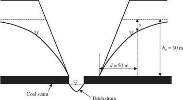
Example 6.4 This example is extracted from Nguyen and Chowdhury (i985). Consider a box cut of an open strip coal mine, as shown in Fig. 6.3. The overburden has a phreatic aquifer overlying the coal seam. In the next bench of operation, excavation is to be made 50 m (d = 50 m) behind the box-cut high wall. It is suggested that for
Figure 6.3 Box cut of an open strip coal mine resulting in water drawdown. (After Nguyen and Chowdhury, 1985.) |
safety reasons of preventing slope instability the excavation should start at the time when the drawdown in the overburden d = 50 m away from the excavation point has reached at least 50 percent of the total aquifer depth (ho).
 |
Nguyen and Raudkivi (1983) gave the transient drawdown equation for this problem as
(6.31)
From the conditional PDF given earlier, the conditional expectation and conditional standard deviation of storage coefficient S, given a specified value of permeability Kh = kh, can be derived, respectively, according to Eqs. (2.110) and (2.111), as
ffs
MSkh = E(SKh = kh) = Ms + Pkh, s—— (kh – Mkh) (6.32)
ffkh
ffskh = ffsy 1 – plh s (6.33)
Therefore, the algorithm for generating bivariate normal random variates to estimate the statistical properties of the drawdown recess time can be outlined as follows:
1. Generate a pair of independent standard normal variates and z’2.
2. Compute the corresponding value of permeability kh = Mkh + ^khZy
3. Based on the value of permeability obtained in step 2, compute the conditional mean and conditional standard deviation of the storage coefficient according to Eqs. (6.32) and (6.33), respectively. Then calculate the corresponding storage coefficient as S = Mskh + ffskhZ2.
4. Use Kh = kh and S = s generated in steps 3 and 4 in Eq. (6.29) to compute the corresponding drawdown recess time t.
5. Repeat steps 1 through 4 n = 400 times to obtain 400 realizations of drawdown recess times {t1, t2,…, t400}.
6. Compute the sample mean, standard deviation, and skewness coefficient of the drawdown recess time according to the last column of Table 2.1.
The histogram ofthe drawdown recess time resulting from 400 simulations is shown in Fig. 6.4. The statistical properties of the drawdown recess time are estimated as
Mean nt = 45.73 days
Standard deviation at = 4.72 days
Skewness coefficient yt = 0.487


Leave a reply