Failure point)

In cases for which several stochastic basic variables are involved in a perfor­mance function, the number of possible combinations of such variables satis­fying W (x) = 0 is infinite. From the design viewpoint, one is more concerned with the combination of stochastic basic variables that would yield the lowest reliability or highest failure probability. The point on the failure surface asso­ciated with the lowest reliability is the one having the shortest distance to the point where the means of the stochastic basic variables are located. This point is called the design point (Hasofer and Lind, 1974) or the most probable failure point (Shinozuka, 1983).

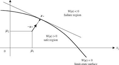
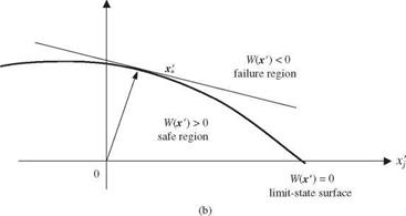
Consider that X = (X1,X2,…,XK)t are K uncorrelated stochastic basic variables having a vector mean px and covariance matrix Dx. The original stochastic basic variables X can be standardized into X’ according to Eq. (4.30). The standardization procedure maps the failure surface in the original x-space onto the corresponding failure surface in x’-space, as shown in Fig. 4.6. Hence the design point in x ‘-space is the one that has the shortest distance from the

Xk (a)

x’ Figure 4.6 Performance function in the original and standardized spaces: (a) original space; (b) standardized space.

failure surface W'(x 0 = 0 to the origin x’ = 0. Such a point can be found by solving

This constrained nonlinear minimization problem can be converted into an unconstrained minimization problem using the Lagrangian function:

Minimize L(x’, %) = (x’tx 7)1/2 + f W'(x’)

in which f is the Lagrangian multiplier, which is unrestricted in sign. The solution to Eq. (4.32) can be obtained by solving the following two equations simultaneously, that is,

in which Vx = (д/д x1, d/dx2,…, d/dxK )t is a gradient operator. FromEq. (4.33a), the design point x * can be expressed as

x * = f * |x *|Vx7 W ‘(x *)

Furthermore, from Eq. (4.34), the distance between the origin x’ = 0 and the design point x * can be obtained as

|x *| = If* ||x *|[VX 7 W ‘(x * )Vx W'(x *)]1/2 = If* ||x *||Vx7 W ‘(x *)| (4.35)

from which the value of the optimal Lagrangian multiplier x* can be determined as

f* = sign[W 7(0)]|Vx W 7( x* )|-1 (4.36)

Substituting Eq. (4.36) into Eq. (4.34) determines the location of the design point as

V W'(x 7)

x* = — sign[W'(O)]|x*| rox * = — sign[W'(0)]|x*|a* (4.37)

|Vx7 W (x *)

in which a* = Vx W 7(x *)/|Vx — W 7(x **)| is a unit vector emanating from the design point x’* and pointing toward the safe region. Referring to Fig. 4.6, where the mean point fux is located in the safe region, hence W'(0) > 0 [or W(px) > 0], and the corresponding — sign[W'(0)]a* is a unit vector emanating from the origin x7 = 0 and pointing to the design point x*. The elements of a* are called the directional derivatives representing the value of the cosine angle between the gradient vector Vx W'(x **) and axes of the standardized variables. Geometri­cally, Eq. (4.37) shows that the vector, x** is perpendicular to the tangent hyper­plane passing through the design point. The shortest distance can be expressed as

Recall that Xk = fik + akX’k, for k = 1, 2,, K. By the chain rule in calculus,

d W'(Xr) d w (X) dXk d w (X)

d Xk ~ d Xk Щ ~ d Xk ak

or in matrix form as

Vx W'(X’) = D^VxW (X) (4.39b)

Then Eq. (4.38) can be written, in terms of the original stochastic basic variables X, as

in which x* = (x1+, x2*,…, xK* )* is the point in the original variable x-space that can be easily determined from the design point x * in x’-space as x* = fix + D У2x *. It will be shown in the next subsection that the shortest distance from the origin to the design point |x *|, in fact, is the absolute value of the reliabil­ity index based on the first-order Taylor series expansion of the performance function W (X) with the expansion point at x*.

Example 4.8 (Linear performance function) Consider that the failure surface is a hyperplane given by

K

W (X) = a + £) akXk

k=1

or in vector form as W(X) = Oq + a* X = 0, with a’s being the coefficients and X being the random variables. Assume that X are uncorrelated random variables with the mean vector fix and covariance matrix Dx. It can be shown that the MFOSM reliability index computed by Eq. (4.29) with /iw = a0 + a* fix and aW = a* Dxa is the AFOSM reliability index.

To show that the original random variables X are first standardized by Eq. (4.30), therefore, in terms of the standardized random variables X’, the preceding linear failure surface can be expressed as

W'(X’) = b0 + b* X’ = 0

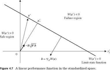
in which bo = Oq + a*fix and b* = a*DУ2. In Fig. 4.7, let the lower half space con­taining the origin of x ‘-space be designated as the safe region. This would require

bj = Oq + a*fix > 0.

Referring to Fig. 4.7, the gradient of W'(X’) is b, which is a vector perpendicular to the failure hyperplane defined by W'(X’) = 0 pointing in the direction of the safe set. Therefore, the vector —a = —bjlb*b is a unit vector emanating from x’ = 0 toward the failure region, as shown in Fig. 4.7. For any vector x’ landing on the

xk

failure hyperplane defined by W'(x’) = 0, the following relationship holds:

—2bl x’ 60

/ЪЪ = TPb

Note that the left-hand side is the length of the vector x’ projected on the unit vec­tor —Ы4¥Ъ, which is the shortest distance from x’ = 0 to the failure hyperplane. Therefore, b0/Vb1 b is the reliability index, that is,

e = 60 = ap + a

ЪЪ л/a Dx a aw

As shown, when the performance function is linear involving uncorrelated stochastic basic variables, the reliability index is the ratio of the expected value of the perfor­mance function to its standard deviation. Furthermore, the MFOSM method would yield the same results as the AFOSM method.

4.1.2 First-order approximation of performance function at the design point

Referring to Eqs. (4.20) and (4.21), the first-order approximation of the perfor­mance function W (X), taking the expansion point xo = x*, is

K

W(X) sk*(Xk — xk*) = s*(X — x*) (4.41)

k=i

in which s* = (sn, s2*,, sK*), a vector of sensitivity coefficients of the per­formance function W (X) evaluated at the expansion point x* that lies on the
limit-state surface, that is,

for k = 1,2,…, K

X=x*

note that W(x*) is not on the right-hand-side of Eq. (4.41) because W(x*) = 0. Hence, at the expansion point x*, the expected value and the variance of the performance function W(X) can be approximated according to Eqs. (4.24) and (4.25) as

f^w ^ s *(Mx x*) (4.42)

al « s CXs* (4.43)

in which fj, x and Cx are the mean vector and covariance matrix of the stochastic basic variables, respectively. If the stochastic basic variables are uncorrelated, Eq. (4.43) reduces to

K

2 _ c.2 „2

aw = Sk*ak

k = 1

in which ak is the standard deviation of the kth stochastic basic variable Xk.

Since a* = s*/|s*|, when stochastic basic variables are uncorrelated, the standard deviation of the performance function W (X) alternatively can be ex­pressed in terms of the directional derivatives as

K

aw = ^2 ak*Sk*ak (4.45)

k=1

where ak* is the directional derivative for the kth stochastic basic variable at the expansion point x*

Sk ak
for k = 1, 2,…, K	(4.46a)

or, in matrix form,

D 1/2Vx W (x*)

| D 1/2Vx W (x*)|

which is identical to the one defined in Eq. (4.37) according to Eq. (4.39). With the mean and standard deviation of the performance function W (X) computed

at x*, the AFOSM reliability index ^afosm given in Eq. (4.34) can be determined as

вafosm = ^ = ^k=1KSk*(lXk — Xk*} (4.47)

Z_jk = 1 ak*sk*Gk

The reliability index eAFOSM also is called the Hasofer-Lind reliability index.

Once the value of eAFOSM is computed, the reliability can be estimated by Eq. (4. 10) as Ps = $^afosm). Since eAFOSM = sign[W40)]|x*|, the sensitiv­ity of eAFOSM with respect to the uncorrelated, standardized stochastic basic variables is

x’

Vx’ eAFOSM = sign[W/(0)]Vx’|x(| = sign[W 40)]—^ = — a* (4.48)

|x *

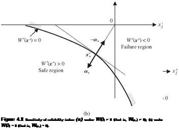
Note that Vx в is a vector showing the direction along which the rate change in the value of the reliability index в increases most rapidly. This direction is indicated by — a* regardless whether the position of the mean of the stochastic basic variables fxx is in the safe region W40) > 0 or failure zone W40) < 0. As shown in Fig. 4.8, the vector — a* points to the failure region, and moving along — a* would result in a more negative-valued W'(x0. This is, geometri­cally, equivalent to pushing the limit-state surface W'(x’) = 0 further away from x’ = 0 in Fig. 4.8a and closer to x’ = 0 in Fig. 4.8b. Hence, moving along the direction of — a* at the design point x* would make the value of the relia­bility index в more positive under W40) > 0, whereas the value of в would be less negative under W40) < 0.

In both cases, the value of the reliability index increases along — a*. Alge­braically, as one moves along — a*, the current value of the limit-state surface W'(x’) changes from 0 to a negative value, that is, W'(x’) = — c, for c > 0. This implies a new limit state for the system defined by W'(x’) = R(x’) — L(x’) + c = 0. The introduction of a positive-valued c in the performance function could mean an increase in resistance, that is, W'(x’) = [R(x0 + c] — L(x’) = 0, or a decrease in load, that is, W'(x’) = R(x’) — [L(x’) — c] = 0. In either case, the reliability index and the corresponding reliability for the system would increase along the direction of — a*.

Equation (4.48) indicates that moving along the direction of a* at the design point x*, the values of the reliability index would decrease and that — ak* is the rate of change in вАго:зМ owing to a one standard deviation change in stochastic basic variable Xk at X = x*. Therefore, the relationship between Vx в and Vxв can be expressed as

or, in matrix form, as

It also can be shown easily that the sensitivity of reliability or failure probability with respect to each stochastic basic variable along the direction of a* can be computed as

ak*ф (eAFOSM) ak* Ф (^afosm) ®k

(4.50a)

or in matrix form as

Vx; Ps = —Ф (eAFOSM)a*

Vx, Ps = Ф (^afosm)Vx, ^afosm = —Ф (^afosm) D x1/2 a*

These sensitivity coefficients would reveal the relative importance of each stochastic basic variable for their effects on reliability or failure probability.