Failure Characteristics
Any system will fail eventually; it is just a matter of time. Owing to the presence of many uncertainties that affect the operation of a physical system, the time the system fails to perform its intended function satisfactorily is random.
5.1.1 Failure density function
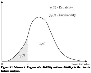
The probability distribution governing the time occurrence of failure is called the failure density function. This failure density function serves as the common thread in the reliability assessments by TTF analysis. Referring to Fig. 5.1, the reliability of a system or a component within a specified time interval (0, t], can be expressed, assuming that the system is operational initially at t = 0, as
|
/ |
TO
ft (t ) dr (5.1a)
in which the TTF is a random variable having ft(t) as the failure density function. The reliability ps (t) represents the probability that the system experiences
 |
no failure within (0, t]. The failure probability, or unreliability, can be expressed as
Pf (t) = P(TTF < t) = 1 – pa(t) = ft(t) dr (5.1b)
0
Note that unreliability pf (t) is the probability that a component or a system would experience its first failure within the time interval (0, t]. As can be seen from Fig. 5.1, as the age of system t increases, the reliability ps(t) decreases, whereas the unreliability pf (t) increases. Conversely, the failure density function can be obtained from the reliability or unreliability as
The TTF is a continuous, nonnegative random variable by nature. Many continuous univariate distribution functions described in Sec. 2.6 are appropriate for modeling the stochastic nature of the TTF. Among them, the exponential distribution, Eq. (2.79), perhaps is the most widely used. Besides its mathematical simplicity, the exponential distribution has been found, both phenomenologically and empirically, to describe the TTF distribution adequately for components, equipment, and systems involving components with a mixture of life distributions. Table 5.1 lists some frequently used failure density functions and their distributional properties.


Leave a reply