Extreme-value distributions

Hydrosystems engineering reliability analysis often focuses on the statisti­cal characteristics of extreme events. For example, the design of flood-control structures may be concerned with the distribution of the largest events over the recorded period. On the other hand, the establishment of a drought- management plan or water-quality management scheme might be interested in the statistical properties of minimum flow over a specified period. Statistics of extremes are concerned with the statistical characteristics of Xmax, n = max{X1, X2,…, Xn} and/or Xmjn,„ = min{X1, X2,…, Xn} in which X1, X2,…, Xn are observations of random processes. In fact, the exact distributions of extremes are functions of the underlying (or parent) distribution that generates the ran­dom observations X1, X2,…, Xn and the number of observations. Of practi­cal interest are the asymptotic distributions of extremes. Asymptotic distribu­tion means that the resulting distribution is the limiting form of Fmax, n(y) or Fmin, n(y) as the number of observations n approaches infinity. The asymptotic distributions of extremes turn out to be independent of the sample size n and the underlying distribution for random observations. That is,

limn^x Fmax, n( y) = Fmax( y) limnxx Fmin, n( y) = Fmin( y)

Furthermore, these asymptotic distributions of the extremes largely depend on the tail behavior of the parent distribution in either direction toward the extremes. The center portion of the parent distribution has little significance for defining the asymptotic distributions of extremes. The work on statistics of extremes was pioneered by Fisher and Tippett (1928) and later was extended

by Gnedenko (1943). Gumbel (1958), who dealt with various useful applications of Xmax, n and Xmin, n and other related issues.

Three types of asymptotic distributions of extremes are derived based on the different characteristics of the underlying distribution (Haan, 1977):

Type I. Parent distributions are unbounded in the direction of extremes, and all statistical moments exist. Examples of this type of parent distribution are normal (for both largest and smallest extremes), lognormal, and gamma distributions (for the largest extreme).

Type II. Parent distributions are unbounded in the direction of extremes, but all moments do not exist. One such distribution is the Cauchy distribution (Sec. 2.6.5). Thus the type II extremal distribution has few applications in practical engineering analysis.

Type III. Parent distributions are bounded in the direction of the desired extreme. Examples of this type of underlying distribution are the beta dis­tribution (for both largest and smallest extremes) and the lognormal and gamma distributions (for the smallest extreme).

Owing to the fact that Xmin, n = — max{-X1, -X2,…, — Xn}, the asymptotic distribution functions of Xmax, n and Xmin n satisfy the following relation (Leadbetter et al., 1983):

Fmin(У) = 1 — Fmax(-y) (2.84)

Consequently, the asymptotic distribution of Xmin can be obtained directly from that of Xmax. Three types of asymptotic distributions of the extremes are listed in Table 2.3.

Extreme-value type I distribution. This is sometimes referred to as the Gumbel distribution, Fisher-Tippett distribution, and double exponential distribution. The CDF and PDF of the extreme-value type I (EV1) distribution have, respec­tively, the following forms:

x — f ~T~
FeV1( x | f, в) = exp ^ — exp	for maxima
(2.85a)
x — f ~T~
for minima
= 1 — exp — exp
+

TABLE 2.3 Three Types of Asymptotic Cumulative Distribution Functions (CDFs) of Extremes Type Maxima Range Minima Range I exp(-e-y) -го < y < ro 1 — exp(-ey) -ro < y < ro II exp( — ya) a < 0, y > 0 1 — exp[ ( y)a] a < 0, y < 0 III exp[ ( y )a ] a > 0, y < 0 1 — exp( — ya) a > 0, y > 0

y

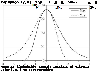
for —to < x, f < to, and P > 0. The shapes of the EV1 distribution are shown in Fig. 2.21, in which transformed random variable Y = (X — f )/p is used. As can be seen, the PDF associated with the largest extreme is a mirror image of the smallest extreme with respect to the vertical line passing through the common mode, which happens to be the parameter f. The first three product-moments of an EV1 random variable are

Px = A1 = f + °.5772p	for the largest extreme
= f — 0.5772P	for the smallest extreme	(2.86a)
= 1.645P2	for both types	(2.86b)
Kx = 1.13955	for the largest extreme
= -1.13955	for the smallest extreme	(2.86c)

The second — to fourth-order L-moments of the EV1 distribution for maxima are A2 = P ln(2) T3 = 0.1699 T4 = 0.1504 (2.87)

Using the transformed variable Y = (X — f )/p, the CDFs of the EV1 for the maxima and minima are shown in Table 2.3. Shen and Bryson (1979) showed

that if a random variable had an EV1 distribution, the following relationship is satisfied when f is small:

where xT is the quantile corresponding to the exceedance probability of 1/T.

Example 2.19 Repeat Example 2.17 by assuming that the annual maximum flood follows the EV1 distribution.

Solution Based on the values of a mean of 6000 ft3/s and standard deviation of 4000 ft3/s, the values of distributional parameters f and в can be determined as follows. For maxima, в is computed from Eq. (2.86b) as

в =

V1.645

and from Eq. (2.86a), one has

f = nQ — 0.577в = 6000 — 0.577(3118.72) = 4200.50 ft3/s

(a) The probability of exceeding 10,000 ft3/s, according to Eq. (2.85a), is

= 1 — exp[- exp(-1.860)]

= 1 — 0.8558 = 0.1442

(b) On the other hand, the magnitude of the 100-year flood event can be calculated as

У100 = g10° — f = — ln[- ln(1 — 0.01)] = 4.60

в

Hence q100 = 4200.50 + 4.60(3118.7) = 18,550 ft3/s.

Extreme-value type III distribution. For the extreme-value type III (EV3) distri­bution, the corresponding parent distributions are bounded in the direction of the desired extreme (see Table 2.3). For many hydrologic and hydraulic ran­dom variables, the lower bound is zero, and the upper bound is infinity. For this reason, the EV3 distribution for the maxima has limited applications. On the other hand, the EV3 distribution of the minima is used widely for modeling the smallest extremes, such as drought or low-flow condition. The EV3 distri­bution for the minima is also known as the Weibull distribution, having a PDF defined as

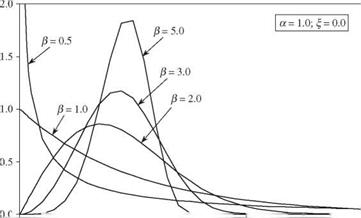
When f = 0 and a = 1, the Weibull distribution reduces to the exponential dis­tribution. Figure 2.22 shows that the versatility of the Weibull distribution function depends on the parameter values. The CDF of Weibull random vari­ables can be derived as

The mean and variance of a Weibull random variable can be derived as

І2 = в (1 — 2-1/a) Г 1 + 1

Generalized extreme-value distribution. The generalized extreme-value (GEV) distribution provides an expression that encompasses all three types of extreme — value distributions. The CDF of a random variable corresponding to the maxi­mum with a GEV distribution is

Fgev(x | f, a, в) = exp	for a = 0	(2.93)
I “————— 1————————— 1————————— f———————————————— і 0.0 0.5 1.0 1.5 2.0 2.5 3.0 x Figure 2.22 Probability density functions of a Weibull random variable.

When a = 0, Eq. (2.93) reduces to Eq. (2.85a) for the Gumbel distribution. For a < 0, it corresponds to the EV2 distribution having a lower bound x > % + в/а, whereas, on the other hand, for a > 0, it corresponds to the EV3 distribution having an upper bound x < % + в/а. For |a| < 0.3, the shape of the GEV distribution is similar to the Gumbel distribution, except that the right-hand tail is thicker for a < 0 and thinner for a > 0 (Stedinger et al., 1993).

The first three moments of the GEV distribution, respectively, are

where sign(a) is +1 or -1 depending on the sign of a. From Eqs. (2.94b) and (2.94c) one realizes that the variance of the GEV distribution exists when a > -0.5, and the skewness coefficient exists when a > -0.33. The GEV distri­bution recently has been used frequently in modeling the random mechanism of hydrologic extremes, such as precipitation and floods.

The relationships between the L-moments and GEV model parameters are