Effect of age on reliability
In general, the reliability of a system or a component is strongly dependent on its age. In other words, the probability that a system can be operational to perform its intended function satisfactorily is conditioned by its age. This conditional reliability can be expressed mathematically as

P(TTF > t, TTF > t + M)
P(TTF > t)
P(TTF > t + M) Ps(t + M) P (TTF > t) = ps(t)
in which t is the age of the system up to the point that the system has not failed, and ps(M 11) is the reliability over a new mission period M, having successfully operated over a period of (0, t ]. In terms of failure rate, ps(M 11) can be written as
|
|||
|
|
||
|
|
||
|
||
|
||

For a process or component following the bathtub failure rate shown in Fig. 5.8 during the useful-life period, the failure rate is a constant, and the failure density function is an exponential distribution. Thus the failure rate h(t) = X. The conditional reliability, according to Eq. (5.13), is
![]() Ps(f i t) = e lt
Ps(f i t) = e lt
which shows that the conditional reliability depends only on the new mission period f regardless of the length of the previous operational period. Hence the time to failure of a system having an exponential failure density function is memoryless.
However, for nonconstant failure rates during the early-life and wear-out periods, the memoryless characteristics of the exponential failure density function no longer hold. Consider the Weibull failure density with a = 1. Referring to Fig. 5.3, the condition a = 1 precludes having a constant failure rate. According to Table 5.1, the conditional reliability for the Weibull failure density function is
As can be seen, ps(f 11) will not be independent of the previous service period t when a = 1. Consequently, to evaluate the reliability of a system for an additional service period in the future during the early-life and wear-out stages, it is necessary to know the length of the previous service period.
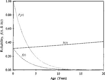
Example 5.4 Refer to Example 5.3. Derive the expression for the conditional reliability and conditional failure density of the 5-mile water main with sandspun cast iron pipe.
Solution Based on the reliability function obtained in Example 5.3, the conditional reliability of the 5-mile sandspun cast iron pipe in the water distribution system can be derived, according to Eq. (5.12), as
![]() ps (t + f )
ps (t + f )
Ps (t)
exp[23.25(1 — e00137(t+f 1)]
exp[23.25(1 — e00137t)]
exp[23.25e00137t(1 – e0 0137f)]
ft(§ 11) = 0.3185 x e0 0137(t+^) x exp[23.25e00137t(1 – e00137^)]
Figure 5.11 shows the conditional reliability and conditional failure density of the pipe system for various service periods at different ages. Note that at age t = 0, the curve simply corresponds to the reliability function.
A commonly used reliability measure of system performance is the mean time to failure (MTTF), which is the expected TTF. The MTTF can be defined mathematically as
Referring to Eq. (2.30), the MTTF alternatively can be expressed in terms of reliability as
0
By Eq. (5.18), the MTTF geometrically is the area underneath the reliability function. The MTTF for some failure density functions are listed in the last column of Table 5.1. For illustration purposes, the MTTFs for some of the components in water distribution systems can be determined from mean time between failures (MTBF) and mean time to repair (MTTR) data listed in Tables 5.2 and 5.3.
Example 5.5 Refer to Example 5.3. Determine the expected elapsed time that a pipe break would occur in the 5-mile sandspun cast iron pipe water main.
Solution The expected elapsed time over which a pipe break would occur can be computed, according to Eq. (5.17), as
f TO f TO
MTTF = ps(t)dt = exp[23.25(1 – e00137t)] dt = 3.015years
00
The main reason for using Eq. (5.18) is purely for computational considerations because the expression for ps(t) is much simpler than ft(t).


Leave a reply