Distributions related to normal random variables

The normal distribution has been playing an important role in the development of statistical theories. This subsection briefly describes two distributions related to the functions of normal random variables.

Figure 2.23 Shapes of standard beta probability density functions. (After Johnson and Kotz, 1972.)

X2 (chi-square) distribution. The sum of the squares of K independent standard normal random variables results in a x2 (chi-square) random variable with K degrees of freedom, denoted as x2- In other words,

E z2 ~ xK (2-101)

k=і

in which the Zks are independent standard normal random variables. The PDF of a x 2 random variable with K degrees of freedom is

f x2(* I K) = 2k/2r1 K/2)x(K/2-1)e-x/2 for x > 0 (2.102)

Comparing Eq. (2.102) with Eq. (2.72), one realizes that the x2 distribution is a special case of the two-parameter gamma distribution with a = K/2 and в = 2. The mean, variance, and skewness coefficient of a xK random variable, respectively, are

ix = K aI = 2 K Yx = 2/v/K72

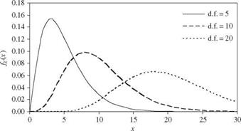
Thus, as the value of K increases, the x2 distribution approaches a symmetric distribution. Figure 2.24 shows a few x2 distributions with various degrees of freedom. If X1, X2,…, XK are independent normal random variables with the common mean ix and variance a2, the x2 distribution is related to the sample of normal random variables as follows:

1. The sum of K squared standardized normal variables Zk = (Xk — X)/ax, k = 1, 2,…, K, has a x2 distribution with (K — 1) degrees of freedom.

2. The quantity (K — 1)S2/a* has a x2 distribution with (K — 1) degrees of freedom in which S2 is the unbiased sample variance computed according to Table 2.1.

Figure 2.24 Shapes of chi-square probability density functions where d. f. refers to the degrees of freedom.

f-distribution. A random variable having a t-distribution results from the ratio of the standard normal random variable to the square root of the x2 random variable divided by its degrees of freedom, that is,

Z

Tk = (2.103)

Xk / K

in which Tk is a t — distributed random variable with K degrees of freedom. The PDF of Tk can be expressed as

Г[( K 4- 1)/21 / r2 -(K+1)/2

f t(r | K) = — + — 1 + for — TO < r < TO (2.104)

1 ж K r( K/2) K

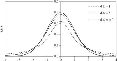
A t-distribution is symmetric with respect to the mean /гг = 0 when K > 1. Its shape is similar to the standard normal distribution, except that the tails of the PDF are thicker than ф(z). However, as K ^to, the PDF of a t — distributed ran­dom variable approaches the standard normal distribution. Figure 2.25 shows some PDFs for t — random variables of different degrees of freedom. It should be noted that when K = 1, the t-distribution reduces to the Cauchy distribu­tion, for which all product-moments do not exist. The mean and variance of a t-distributed random variable with K degrees of freedom are

!i:r = 0 ol = K/(K — 2) for K > 3

When the population variance of normal random variables is known, the sample mean X of K normal random samples from N(p. r, o^) has a normal distribu­tion with mean /гг and variance ol /K. However, when the population variance is unknown but is estimated by S2 according to Table 2.1, then the quantity VK(X — /гг )/S, which is the standardized sample mean using the sample vari­ance, has a t-distribution with (K — 1) degrees of freedom.

t Figure 2.25 Shapes of t-distributions where d. f. refers to degrees of freedom.