Classifications of Random Variates Generation Algorithms
Let a random variable X have the cumulative distribution function (CDF) Fx(x). From Sec. 2.3.1, Fx(x) is a nondecreasing function with respect to the value of x, and 0 < Fx(x) < 1. Therefore, F-1(u) may be defined for any value of u between 0 and 1 as F-1(u) is the smallest x satisfying Fx(x) > u.
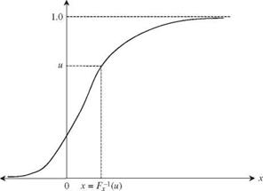
For the majority of continuous probability distributions applied in hydrosystems engineering and analysis, Fx(x) is a strictly increasing function of x. Hence a unique relationship exists between Fx (x) and u; that is, u = Fx (x), as shown in Fig. 6.1. Furthermore, it can be shown that if U is a standard uniform random variable defined over the unit interval [0, 1], denoted by U ~ U(0,1), the following relationship holds:
X = Fx-1(U) (6.6)
Note that X is a random variable because it is a function of the random variable U. From Eq. (6.6), the one-to-one correspondence between X and U, through the CDF, enables the generation of random numbers X ~ Fx(x) from the standard uniform random numbers. The algorithm using the CDF-inverse method for generating continuous random numbers from a CDF Fx(x) can be stated as follows:
1. Generate n uniform random numbers u1, u2,…, un from U(0,1).
2. Solve for xi = F-1(ui), for і = 1, 2,…, n.
|
Fx(x) = u
Figure 6.1 Schematic diagram ofthe inverse-CDF method for generating random variates. |
Example 6.1 Consider that the Manning roughness coefficient X of a cast iron pipe is uncertain, having a uniform distribution fx(x) = 1/(6 — a), a < x < b. Develop an algorithm using the CDF-inverse method to generate a random Manning roughness coefficient.
 |
 |
Solution Using the CDF-inverse method, the expression of the CDF of the random variable is first sought. The CDF for this example can be derived as
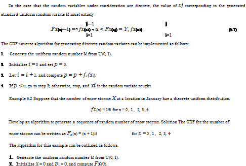
3. Test if pi < u < Fx(x). If yes, x is the solution; otherwise, go to step 4.
4. Let p1 = Fx(x), x = x + 1, and compute Fx(x + 1). Go to step 3.
To apply the CDF-inverse method for generating random numbers efficiently, an explicit expression between X and U is essential so that X can be obtained analytically from the generated U. The distributions the inverse forms of which are analytically expressible include exponential, uniform, Weibull, and Gumbel. Table 6.3 lists some distributions that are used in hydrosystems the CDF inverses of which are analytically expressible.
When the analytical forms of the CDF inverse are not available, applying the CDF-inverse method would require solving
|
/ |
x
fx (t) dt (6.8)
-TO
for x from the known u. For many commonly used distributions such as normal, lognormal, and gamma, solving Eq. (6.8) is inefficient and difficult. More efficient algorithms have been developed to generate random variates from those distributions; some of these are described in Sec. 6.4.


Leave a reply