Algorithms of AFOSM for independent normal parameters

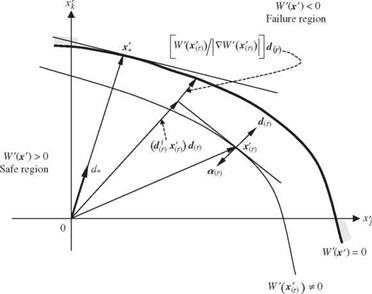
Hasofer-Lind algorithm. In the case that X are independent normal stochastic basic variables, standardization of X according to Eq. (4.30) reduces them to independent standard normal random variables Z’ with mean 0 and covariance matrix I, with I being a K x K identity matrix. Referring to Fig. 4.8, based on the geometric characteristics at the design point on the failure surface, Hasofer and Lind (1974) proposed the following recursive equation for determining the design point z (.

in which subscripts (r) and (r + 1) represent the iteration numbers, and —a denotes the unit gradient vector on the failure surface pointing to the failure region. Referring to Fig. 4.9, the first terms of Eq. (4.51), — (—al(r z(r))a(r), is a projection vector of the old solution vector z (r) onto the vector —a (r) emanating from the origin. The quantity W'(z(r))/|VW'(z(r))| is the step size to move from W'(z(r)) to W'(z’) = 0 along the direction defined by the vector —a(r). The second term is a correction that further adjusts the revised solution closer to the limit-state surface. It would be more convenient to rewrite the preceding recursive equation in the original лт-space as

Based on Eq. (4.52), the Hasofer-Lind AFOSM reliability analysis algorithm for problems involving uncorrelated, normal stochastic variables the can be outlined as follows:

Step 1: Select an initial trial solution x(r).

Step 2: Compute W(x(r>) and the corresponding sensitivity coefficient vector

s (r).

Step 3: Revise solution point x(r+1), according to Eq. (4.52).

Step 4: Check if x(r) and x(r+1) are sufficiently close. If yes, compute the reli­ability index eAFOSM according to Eq. (4.47) and the corresponding reliability

Figure 4.9 Geometric interpretation of Hasofer-Lind algorithm in standard­ized space.

ps = ФС^їге^; then, go to step 5. Otherwise, update the solution point by letting x(r) = x(r+1> and return to step 2.

Step 5: Compute the sensitivity of the reliability index and reliability with respect to changes in stochastic basic variables according to Eqs. (4.48), (4.49), and (4.50).

It is possible that a given performance function might have several design points. In the case that there are J such design points, the reliability can be calculated as

Ps = №(^afosm)]J (4.53)

Ang-Tang algorithm. The core of the updating procedure of Ang and Tang (1984) relies on the fact that according to Eq. (4.47), the following relationship should be satisfied:

K

У> (pk — Xk> — ak>P*vk) = 0 (4.54)

k=1

Since the variables X are random and uncorrelated, Eq. (4.35) defines the fail­ure point within the first-order context. Hence Eq. (4.47) can be decomposed into

Xk = Pk — ak>в*°k for k = 1, 2,…, K

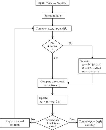
Ang and Tang (1984) present the following iterative procedure to locate the de­sign point x+ and the corresponding reliability index ^AFOSM under the condition that stochastic basic variables are independent normal random variables. The Ang-Tang AFOSM reliability algorithm for problems involving uncorrelated normal stochastic variables has the following steps (Fig. 4.10):

Step 1: Select an initial point x(r) in the parameter space. For practicality, the point iix where the means of stochastic basic variables are located is a viable starting point.

Figure 4.10 Flowchart of the Ang-Tang AFOSM reliability analysis involving uncorre­lated variables.

Step 2: At the selected point x (r), compute the mean of the performance func­tion W (X) by

MW = w(x(r)) + s r)(^x — x(r)) (4.56)

and the variance according to Eq. (4.44).

Step 3: Compute the corresponding reliability index ) according to Eq. (4.34).

Step 4: Compute the values of directional derivative ak for all k = 1, 2,, K according to Eq. (4.46).

Step 5: Revise the location of expansion point x(r+p according to Eq. (4.56) using ak and в(г) obtained from steps 3 and 4.

Step 6: Check if the revised expansion point x(r +p differs significantly from the previous trial expansion point x (r). If yes, use the revised expansion point as the new trial point by letting x(r) = x(r+p, and go to step 2 for an additional iteration. Otherwise, the iteration procedure is considered complete, and the latest reliability index is eAFOSM and is to be used in Eq. (4.10) to compute the reliability ps.

Step 7: Compute the sensitivity of the reliability index and reliability with respect to changes in stochastic basic variables according to Eqs. (4.48), (4.49), and (4.50).

Referring to Eq. (4.8), the reliability is a monotonically increasing function of the reliability index в, which, in turn, is a function of the unknown failure point. The task to determine the critical failure point x+ that minimizes the reliability is equivalent to minimizing the value of the reliability index в. Low and Tang (1997), based on Eqs. (4.31a) and (4.31b) developed an optimization procedure in Excel by solving

Mm в = ^J(x — fxxУC-1(x — fxx) 57)

subject to W(x) = 0

Owing to the nature of nonlinear optimization, both AFOSM-HL and AFOSM — AT algorithms do not necessarily converge to the true design point associated with the minimum reliability index. Madsen et al. (1986) suggested that dif­ferent initial trial points be used and that the smallest reliability index be cho­sen to compute the reliability. To improve the convergence of the Hasofer-Lind algorithm, Liu and Der Kiureghian (1991) proposed a modified objective func­tion for Eq. (4.31a) using a nonnegative merit function.

Example 4.9 (Uncorrelated, normal) Refer to Example 4.5 for a storm sewer relia­bility analysis problem with the following data:

Variable	Mean	Coefficient of variation
n (ft1/6)	0.015	0.05
D (ft)	3.0	0.02
S (ft/ft)	0.005	0.05

Assume that all three stochastic basic variables are independent normal random variables. Compute the reliability that the sewer can convey an inflow discharge of 35 ft3/s using the AFOSM-HL algorithm.

Solution The initial solution is taken to be the means of the three stochastic basic variables, namely, x(1) = fix = (^n, xd, xs)t = (0.015, 3.0, 0.005^. The covariance matrix for the three stochastic basic variables is

		0	0		0.000752	0	0
D x =	0 0	D 0	0 aS.	=	0 0	0.062 0	0 0.000252

For this example, the performance function Qc — Ql is

W(n, D, S) = Qc — Ql = 0.463n—1D8/3S1/2 — 35

Note that because the W(^n, гD, XS) = 6.010 > 0, the mean point fix is located in the safe region. At x(1) = fix, the value of the performance function W(n, D, S) = 6.010, which is not equal to zero. This implies that the solution point x(1), does not lie on the limit-state surface. By Eq. (4.52), the new solution x(2) can be obtained as x(2) = (0.01592,2.921,0.004847). Then one checks the difference between the two consecutive solution points as

5 = |x (1) — x (2)| = [(0.01592 — 0.015)2 + (2.921 — 3.0)2 + (0.004847 — 0.005)2]05 = 0.07857

which is considered large, and therefore, the iteration continues. The following table lists the solution point x(r), its corresponding sensitivity vector s(r), and the vector of directional derivatives a (r) in each iteration. The iteration stops when the differ­ence between the two consecutive solutions is less than 0.001 and the value of the performance function is less than 0.001.

Iteration	Var.	x (r )	s (r )		a(r)	x(r+1)
r = 1	n	0.1500 x 10—01	—0.2734 x 10+04		—0.6468 x 10+00	0.1592 x 10—01
	D	0.3000 x 10—01	0.3650 x 10+02		0.6907 x 10+00	0.2921 x 10+01
	S	0.5000 x 10—02	0.4101 x 10+04		0.3234 x 10+00	0.4847 x 10—02
		5 = 0.7857 x 10—01	W = 0.6010 x 10+01	в =	0.0000 x 10+00
r = 2	n	0.1592 x 10—01	—0.2226 x 10+04		—0.6138 x 10+00	0.1595 x 10—01
	D	0.2921 x 10+01	0.3239 x 10+02		0.7144 x 10+00	0.2912 x 10+01
	S	0.4847 x 10—02	0.3656 x 10+04		0.3360 x 10+00	0.4827 x 10—02
		5 = 0.9584 x 10—02	W = 0.4421 x 10+00	в =	0.1896 x 10+01

(Continued)

Iteration	Var.	x (r )	s (r )		a(r)	x(r+1)
r = 3	n	0.1595 x 10—01	—0.2195 x 10+04		—0.6118 x 10+00	0.1594 x 10—01
	D	0.2912 x 10—01	0.3209 x 10+02		0.7157 x 10+00	0.2912 x 10+01
	S	0.4827 x 10—02	0.3625 x 10+04		0.3369 x 10+00	0.4827 x 10—02
		S = 0.1919 x 10—03	W = 0.2151 x 10—02	в	= 0.2056 x 10+01
r = 4	n	0.1594 x 10—01	—0.2195 x 10+04		—0.6119 x 10+00	0.1594 x 10—01
	D	0.2912 x 10+01	0.3210 x 10+02		0.7157 x 10+00	0.2912 x 10+01
	S	0.4827 x 10—02	0.3626 x 10+04		0.3369 x 10+00	0.4827 x 10—02
		S = 0.3721 x 10—05	W = 0.2544 x 10—06	в	= 0.2057 x 10+01

After four iterations, the solution converges to the design point x* = (n*, D*, S*)г = (0.01594, 2.912, 0.004827)г. At the design point x*, the mean and standard deviation ofthe performance function W canbe estimated, by Eqs. (4.42) and (4.43), respectively, as

pw* = 5.536 and aw* = 2.691

The reliability index then can be computed as в* = IW/&w* = 2.057, and the corre­sponding reliability and failure probability can be computed, respectively, as

ps = Ф(в*) = 0.9802 pf = 1 — ps = 0.01983

Finally, at the design point x*, the sensitivity of the reliability index and reliabil­ity with respect to each of the three stochastic basic variables can be computed by Eqs. (4.49) and (4.50). The results are shown in columns (4) to (7) ofthe following table:

Variable (1)	x* (2)	a* (3)	9в/9 X (4)	9ps/9 X (5)	9в/9 x (6)	9 ps/9 x (7)	хдв/в’д X (8)	хдps/ps 9x (9)
n	0.01594	— 0.6119	0.6119	0.02942	815.8	39.22	6.323	0.638
D	2.912	0.7157	—0.7157	—0.03441	—11.9	—0.57	—16.890	—1.703
S	0.00483	0.3369	— 0.3369	— 0.01619	—1347.0	—64.78	—3.161	—0.319

From the preceding table, the quantities 9в/9х’к and 9ps/9x’k show the sensitivity of the reliability index and reliability for one standard deviation change in the k-th stochastic basic variable, whereas 9в/9Xk and 9ps/9Xk correspond to one unit change of the k-th stochastic basic variables in the original space. As can be seen, the sensitivity of в and ps associated with Manning’s roughness coefficient is positive, whereas those for pipe size and slope are negative. This indicates that an increase in Manning’s roughness coefficient would result in an increase in в and ps, whereas an increase in slope and/or pipe size would decrease в and ps. The indication is confusing from a physical viewpoint because an increase in Manning’s roughness coefficient would decrease the flow-carrying capacity of the sewer, whereas, on the other hand, an increase in pipe diameter and/or pipe slope would increase the sewer’s conveyance capacity. The problem is that the sensitivity coefficients for в and ps are taken relative to the design point on the failure surface; i. e., a larger Manning’s would be farther from the system’s mean condition, thus resulting in a larger value of в. However, larger values ofpipe diameter or slope would be closer to the system’s mean condition, thus resulting in a smaller value of в. Thus the sign of the sensitivity coefficients is deceiving, but their magnitude is useful, as described in the following paragraphs.

Furthermore, one can judge the relative importance of each stochastic basic vari­able based on the absolute values of the sensitivity coefficients. It is generally difficult to draw a meaningful conclusion based on the relative magnitude of дв/дx and дps/dx because units of different stochastic basic variables are not the same. Therefore, sensi­tivity measures not affected by the dimension of the stochastic basic variables, such as дв/дx’ and дps/дx’, generally are more useful. With regard to a one standard deviation change, for example, pipe diameter is significantly more important than pipe slope.

An alternative sensitivity measure, called the relative sensitivity or the partial elasticity (Breitung, 1993), is defined as