AFOSM reliability analysis for nonnormal correlated stochastic variables

For most practical engineering problems, parameters involved in load and re­sistance functions are correlated nonnormal random variables. Such distribu­tional information has important implications for the results of reliability com­putations, especially on the tail part of the distribution for the performance function. The procedures of the Rackwitz normal transformation and orthogo­nal decomposition described previously can be incorporated into AFOSM reliability analysis. The Ang-Tang algorithm, outlined below, first performs the orthogonal decomposition, followed by the normalization, for problems involv­ing multivariate nonnormal stochastic variables (Fig. 4.12).

The Ang-Tang AFOSM algorithm for problems involving correlated nonnor­mal stochastic variables consists of the following steps:

Step 1: Decompose correlation matrix Rx to find its eigenvector matrix Vx and eigenvalues Лх using appropriate techniques.

Step 2: Select an initial point x(r) in the original parameter space.

Step 3: At the selected point x(r), compute the mean and variance of the performance function W(X) according to Eqs. (4.56) and (4.43), respectively.

Step 4: Compute the corresponding reliability index во-) according to Eq. (4.8).

Step 5: Compute the mean pkN,(r) and standard deviation akN,(r) of the normal equivalent using Eqs. (4.60) and (4.61) for the nonnormal stochastic variables.

Step 6: Compute the sensitivity coefficient vector with respect to the per­formance function sz>,(r) in the independent, standardized normal z’-space, according to Eq. (4.68), with Dx replaced by DxN,(r).

Step 7: Compute the vector of directional derivatives a? (r) according to Eq. (4.67).

Step 8: Using во-) and a^ ,о) obtained from steps 4 and 7 , compute the location of solution point z(r +in the transformed domain according to Eq. (4.70).

Step 9: Convert the obtained expansion point z(r+1) back to the original pa­rameter space as

x (r + 1) = px, N,(r) + D x, N,(r) Vx ЛУ2 z (r +1) (4.73)

in which px, N,(r) is the vector of means of normal equivalent at solution point x(r), and Dx, N,(r) is the diagonal matrix of normal equivalent variances.

Step 10: Check if the revised expansion point x(r+1) differs significantly from the previous trial expansion point x (r). If yes, use the revised expansion point as the trial point by letting x(r) = x(r+1), and go to step 3 for another iteration. Otherwise, the iteration is considered complete, and the latest reliability index во) is used in Eq. (4.10) to compute the reliability ps.

Step 11: Compute the sensitivity of the reliability index and reliability with respect to changes in stochastic variables according to Eqs. (4.48), (4.49), (4.51), (4.69), and (4.58), with Dx replaced by D x, n at the design point x^.

One drawback of the Ang-Tang algorithm is the potential inconsistency be­tween the orthogonally transformed variables U and the normal-transformed space in computing the directional derivatives in steps 6 and 7. This is so be­cause the eigenvalues and eigenvectors associated with Rx will not be identical to those in the normal-transformed variables. To correct this inconsistency, Der Kiureghian and Liu (1985), and Liu and Der Kiureghian(1986) developed a
normal transformation that preserves the marginal probability contents and the correlation structure of the multivariate nonnormal random variables.

Suppose that the marginal PDFs of the two stochastic variables Xj and Xk are known to be f j (Xj) and fk (xk), respectively, and their correlation coefficient is pjk. For each individual random variable, a standard normal random variable that satisfies Eq. (4.59) is

Ф( Zj) = Fj (Xj) Ф( Zk) = Fk (Xk) (4.74)

By definition, the correlation coefficient between the two stochastic variables X j and Xk satisfies

Xj J j f Xk Jk
G	Gk
(4.75)
Xj Xj f Xk ixk Gk
fj, k (Xj, Xk) dxj dxk

where xk and Gk are, respectively, the mean and standard deviation of Xk. By the transformation of variable technique, the joint PDF f j, k (Xj, Xk) in Eq. (4.75) can be expressed in terms of a bivariate standard normal PDF as dj dn

д X j d Xk d Zk d Zk d Xj d Xk

where ф(Zj, zk | pjk ) is the bivariate standard normal PDF for Zj and Zk having zero means, unit standard deviations, and correlation coefficient pjk, and the elements in Jacobian matriX can be evaluated as

dZk _ дф—^ЫУ] _ fk (Xk) dXk dXk Ф (Zk )

Then the joint PDF of Xj and Xk can be simplified as

fj I Xj, Xk) = HZ,,Zk |pjk) — ф^ Фф* 14.76)

Substituting Eq. (4.76) into Eq. (4.75) results in the Nataf bivariate distribution model (Nataf, 1962):

in which Xk = F— 1 [Ф (Zk)].

Two conditions are inherently considered in the bivariate distribution model of Eq. (4.77):

1. According to Eq. (4.74), the normal transformation satisfies,

Zk — ф-^Fk (Xk)] for k — 1,2,…, K (4.78)

This condition preserves the probability content in both the original and the standard normal spaces.

2. The value of the correlation coefficient in the normal space lies between -1 and +1.

For a pair of nonnormal stochastic variables Xj and Xk with known means ц j and nk, standard deviations oj and ok, and correlation coefficient pjk, Eq. (4.77) can be applied to solve for pjjk. To avoid the required computation for solving pjjk in Eq. (4.74), Der Kiureghian and Liu (1985) developed a set of semiempirical formulas as

pjk — Tjkpjk (4.79)

in which Tjk is a transformation factor depending on the marginal distributions and correlation of the two random variables considered. In case both the random variables under consideration are normal, the transformation factor Tjk has a value of 1. Given the marginal distributions and correlation for a pair of random variables, the formulas of Der Kiureghian and Liu (1985) compute the corresponding transformation factor Tjk to obtain the equivalent correlation pjk as if the two random variables were bivariate normal random variables. After all pairs of stochastic variables are treated, the correlation matrix in the correlated normal space Rz is obtained.

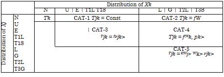
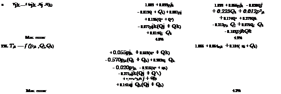
Ten different marginal distributions commonly used in reliability computa­tions were considered by Der Kiureghian and Liu (1985) and are tabulated in Table 4.4. For each combination of two distributions, there is a corresponding formula. Therefore, a total of 54 formulas for 10 different distributions were developed, and they are divided into five categories, as shown in Fig. 4.13. The complete forms of these formulas are given in Table 4.5. Owing to the semiem­pirical nature of the equations in Table 4.5, it is a slight possibility that the resulting pjk may violate its valid range when pjk is close to -1 or +1.

Based on the normal transformation of Der Kiureghian and Liu, the AFOSM reliability analysis for problems involving multivariate nonnormal random variables can be conducted as follows:

Step 1: Apply Eq. (4.77) or Table 4.5 to construct the correlation matrix Rz for the equivalent random variables Z in the standardized normal space.

Step 2: Decompose correlation matrix Rz to find its eigenvector matrix Vz and eigenvalues Xz’s using appropriate orthogonal decomposition techniques. Therefore, Z’ — Л-1/2 VzZ is a vector of independent standard normal ran­dom variables.

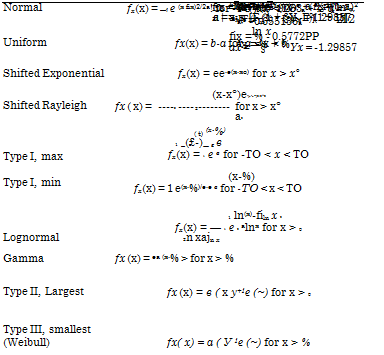
TABLE 4.4 Definitions of Distributions Used in Fig. 4.13 and Table 4.5

Distributions PDF

Note:

N = Normal

U = Uniform

E = Shifted exponential

T1L = Type 1 largest

pk = Correlation coefficient

Figure 4.13 Categories of the normal transformation factor Tjk — (After Der Kiureghi-n and Liu, 1985).

TABLE 4.5 Semiempirical Normal Transformation Formulas (a) Category 1 of the transformation factor j in Fig. 4.13 U E R T1L T1S N Tjk = constant 1.023 1.107 1.014 1.031 1.031 Max. error 0.0% 0.0% 0.0% 0.0% 0.0% NOTE: Distribution indices are N = normal; U = uniform; E = shifted exponential; R = shifted Rayleigh; T1L = type 1, largest value; T1S = type 1, smallest value.

(b)
Category 2 of the transformation factor Tjk in Fig. 4.13

	L	G	T2L	T3S
Tjk = f (Qk) N Max. error	Qk	1.001 — 1.007Qk + 0.118Q 0.0%	1.030 + 0.238Qk + 0.364Q 0.1%	1.031 — 0.195Qk + 0.328Qk 0.1%
Zln(1+Qk) Exact
NOTE: Qk is the coefficient of variation of the j th variable; distribution indices are N type 3, smallest value. SOURCE: After Der Kiureghian and Liu (1985).	= normal; L = lognormal; G = gamma; T2L	= type 2, largest value; T3S =

(Continued)

		U	E	R	T1L	T1S
U	Tjk = f(Pjk)	1.047 — 0.047pjk	1.133 + 0.029pjk	1.038 — 0.008p2k	1.055 + 0.015p2k	1.055 + 0.015p2k
	Max. error	0.0%	0.0%	0.0%	0.0%	0.0%
E	Tjk = f(Pjk)		1.229 — 0.367pjk	1.123 — 0.100pjk	1 . 142 — 0 . 154 p jk	1.142 + 0.154p jk
			+ °.153p! k	+ 0.021p|k	+ 0.031p|k	+ °.°31p2k
	Max. error		1.5%	0.1%	0.2%	0.2%
R	Tjk = f(Pjk)			1.028 — 0.029pjk	1 . 046 — 0 . 045 p jk	1.046 + 0.045p jk
					+ 0.006p2k	+ 0.006p2jk
	Max. error			0.0%	0.0%	0.0%
T1L	Tjk = f(Pjk)				1.064 — 0.069pjk	1.064 + 0.069p jk
					+ 0.005pj	+ 0.005pjk
	Max. error				0.0%	0.0%
T1S	Tjk = f(Pjk)					1.064 — 0.069pjk
						+ 0.005p2k
	Max. error					0.0%

TABLE 4.5 Semiempirical Normal Transformation Formulas (Continued) (c) Category 3 of the transformation factor Tjk in Fig. 4.11

NOTE: pjk is the correlation coefficient between the j th variable and the kth variable; distribution indices are U = uniform; E = shifted exponential; R = shifted Rayleigh; T1L = type 1, largest value; T1S = type 1, smallest value.

		L	G	T2L	T3S
U	Tjk — f(pjk, Qk )	1.019 + 0.014Qk + 0.010p2k + 0.249Q2	1.023 — 0.007Qk + 0.002p2k + 0.127Q?	1.033 + 0.305Qk + 0.074p2k + 0.405Qk	1.061 — 0.237Qk — 0.005p2jk + 0.379Q?
	Max. error	0.7%	0.1% k	2.1% k	0.5% k
E	Tjk — f (pjk, Qk )	1.098 + 0.003pjk + 0.019Qk + 0.025p2k + 0.303Q2 — 0.437pjkQk	1.104 + 0.003pjk — 0.008Qk + 0.014p2k + 0.173Qk — 0.296pjkQk	1.109 — 0.152pjk + 0.361Qk + 0.130p2k + 0.455 Q2 — 0.728pjkQk	1.147 + 0.145pjk — 0.271Qk + 0.010p2k + 0.459Qk — 0.467pjkQk
	Max. error	1.6%	0.9%	0.9%	0.4%
R	Tjk — f (pjk, Qk )	1.011 + 0.001pjk + 0.014Qk + 0.004p2k + 0.231Qk — 0.130pjkQk	1.014 + 0.001pjk — 0.007Qk + 0.002p2k + 0.126Qk — 0.090pjkQk	1.036 — 0.038pjk + 0.266Qk + 0.028p2k + 0.383 Qk — 0.229pjkQk	1.047 + 0.042pjk — 0.212Qk + 0.353Qk — 0.136pjkQk
	Max. error	0.4%	0.9%	1.2%	0.2%
T1L	Tjk — f (pjk, Qk )	1.029 + 0.001pjk + 0.014Qk + 0.004p2k + 0.233Qk -0.197pjkQk	1.031 + 0.001pjk — 0.007Qk + 0.003p2k + 0.131Qk -0.132pjkQk	1.056 — 0.060pjk + 0.263Qk + 0.020p2k + 0.383 Qk -0.332p jkQk	1.064 + 0.065pjk — 0.210Qk + 0.003p2k + 0.356Qk -0.211pjkQk
	Max. error	0.3%	0.3%	1.0%	0.2%
T1S	Tjk — f (pjk, Qk )	1.029 + 0.001pjk + 0.014Qk + 0.004p2k + 0.233Qk + 0.197p jkQk	1.031 — 0.001pjk — 0.007Qk + 0.003p2k + 0.131Qk + 0.132pjk Qk	1.056 + 0.060pjk + 0.263Qk + 0.020p2jk + 0.383 Qk + °.332pjk Qk	1.064 — 0.065pjk — 0.210Qk + 0.003p2k + 0.356Qk + 0.211p jkQk
	Max. error	0.3%	0.3%	1.0%	0.2%

NOTE: pjk is the correlation coefficient between the j th variable and the kth variable; Qk is the coefficient of variation of the kth variable; distribution indices are U = uniform; E = shifted exponential; R = shifted Rayleigh; T1L = type 1, largest value; T1S = type 1, smallest value; L = lognormal; G = gamma; T2L = type 2, largest value; T3S = type 3 smallest value.

(Continued)

TABLE 4.5 Semiempirical Normal Transformation Formulas (Continued) (e) Category 5 of the transformation factor Tjk in Fig. 4.13
L G T2L T3S
Tjk — f (pjk, Qk) ——— 1п(1+р-^ ak) 1.001 + 0.033pjk + 0.004Qj pjky 1n 0+j ln(1+Qk) — 0.016^k + 0.002pjk + 0.223Q2 + 0.130^k — 0.104pjkQj + 0.029Ц; Qk — 0.119pjk&k Max. error Exact 4.0%
1.026 + 0.082pjk — 0.019Qj — 0.222Qk + 0.018pjk + 0.288Q2 + 0.379Q2 — 0.104pjkQj + 0.12601 j Qk — 0.277pjkQk 4.3%	1.31 + 0.052pjk + 0.011Q j — 0.21Qk + 0.002p2k + 0.22Q2 + 0.35Qk + 0.005pQj- + 0.009Qj Qk — 0.174pQk 2.4% 1.32 + 0.034pjk — 0.007Qj — 0.202Qk + 0.121Q2 + 0.339Q2 — 0.006pQj + 0.003Q7^ Qk — 0.111pQk 4.0% 1.065 + 0.146pjk + 0.241Q j — 0.259Qk + 0.013p2k + 0.372Q2 + 0.435Q2 + 0.005pQj- + 0.034Qj Qk — 0.481pQk
L
3.8%
1.063 — 0.004pjk — 0.200(Qj + Qk) — 0.001pj + 0.337(Q2 + Qk) + 0.007p(Qj + Qk) — 0.007Qj Qk 2.62%
T3S Tjk — f (pjk ,Qj, Qk)
Max. error
NOTE: pjk is the correlation coefficient between the jth variable and the kth variable; Qj is the coefficient of variation of the j th variable; Qk is the coefficient of variation of the kth variable; distribution indices are L — lognormal; G — gamma; T2L — type 2, largest value; T3S — type 3, smallest value.

Step 3: Select an initial point x(r) in the original parameter space X, and com­pute the sensitivity vector for the performance function sx,(r) = VxW(x(r>).

Step 4: At the selected point x(r), compute the means (j, N,(r) = (p.1N, p.2N,…, IJ-knY and standard deviations aN,(r) = (o1N, o2N,…, oKN)1 of the normal equivalent using Eqs. (4.59) and (4.60) for the nonnormal stochastic variables. Compute the corresponding point zr) in the independent standardized nor­mal space as

in which Dx, N,(r) = diag(o2N, o^N,…, oKN), a diagonal matrix containing the variance of normal equivalent at the selected point x(r). The correspond­ing reliability index can be computed as fi(r) = sign[W/(0)]|z(r)|.

Step 5: Compute the vector of sensitivity coefficients for the performance function in Z’-space sz>,(r) = Vz> W(zr)), by Eq. (4.68), with Dx replaced by D x, n,(r), and x and &x replaced by V’z and Л^, respectively. Then the vector of directional derivatives in the independent standard normal space az ,(r) can be computed by Eq. (4.67).

Step 6: Apply Eq. (4.51) of the Hasofer-Lind algorithm or Eq. (4.70) of the Ang-Tang algorithm to obtain a new solution z (r +1).

Step 7: Convert the new solution z(r+1) back to the original parameter space by Eq. (4.66a), and check for convergence. If the new solution does not satisfy convergence criteria, go to step 3; otherwise, go to step 8.

Step 8: Compute the reliability, failure probability, and their sensitivity vec­tors with respect to change in stochastic variables.

Note that the previously described normal transformation of Der Kiureghian and Liu (1985) preserves only the marginal distributions and the second-order correlation structure of the correlated random variables, which are partial statistical features of the complete information represented by the joint dis­tribution function. Regardless of its approximate nature, the normal transfor­mation of Der Kiureghian and Liu, in most practical engineering problems, rep­resents the best approach to treat the available statistical information about the correlated random variables. This is so because, in reality, the choices of multivariate distribution functions for correlated random variables are few as compared with univariate distribution functions. Furthermore, the derivation of a reasonable joint probability distribution for a mixture of correlated non­normal random variables is difficult, if not impossible. When the joint PDF for the correlated nonnormal random variables is available, a practical normal transformation proposed by Rosenblatt (1952) can be viewed as the generaliza­tion of the normal transformation described in Sec. 4.5.5 for the case involving independent variables. Notice that the correlations among each pair of ran­dom variables are implicitly embedded in the joint PDF, and determination of correlation coefficients can be made according to Eqs. (2.47) and (2.48).

The Rosenblatt method transforms the correlated nonnormal random vari­ables X to independent standard normal random variables Z’ in a manner similar to Eq. (4.78) as

z[ = Ф ЧFi(xi)] z2 = Ф-1[F2(X2 |xi)]

zk = Ф 1[Fk(Xk|xi, X2, Xk-i)]

z’K = Ф 1[Fk(XK|Xi, X2,Xk—1)]

in which Fk(Xk |Xi, X2,, Xk—i) = P(Xk < Xk |x1, X2,…, Xk—i) is the conditional CDF for the random variable Xk conditional on X1 = X1, X 2 = X2,…, Xk—1 = Xk—1. Based on Eq. (2.17), the conditional PDF fk (Xk X2,…, Xk—1) for the random variable Xk can be obtained as

with f (x1,X2,…,Xk—1,Xk) being the marginal PDF for X1,X2,…,Xk—1,Xk; the conditional CDF Fk(xk |x1, x2,…, xk—1) then can be computed by

To incorporate the Rosenblatt normal transformation in the AFOSM algo­rithms described in Sec. 4.5.5, the marginal PDFs fk (xk) and the conditional CDFs Fk(xk|x1, x2,…, xk—1), for k = 1, 2,…, K, first must be derived. Then Eq. (4.81) can be implemented in a straightforward manner in each itera­tion, within which the elements of the trial solution point x(r) are selected successively to compute the corresponding point in the equivalent independent standard normal space z(rand the means and variances by Eqs. (4.80) and (4.81), respectively. It should be pointed out that the order of selection of the stochastic basic variables in Eq. (4.81) can be arbitrary. Madsen et al. (1986, pp. 78-80) show that the order of selection may affect the calculated failure probability, and their numerical example does not show a significant difference in resulting failure probabilities.