Acceptance-rejection methods
Consider a problem for which random variates are to be generated from a specified probability density function (PDF) fx(x). The basic idea of the
|
TABLE 6.3 List of Distributions the Cumulative Distribution Function (CDF) Inverses of which Are Analytically Expressible
|
acceptance-rejection (AR) method is to replace the original fx(x) by an appropriate PDF hx(x) from which random variates can be produced easily and efficiently. The generated random variate from hx(x), then, is subject to testing before it is accepted as one from the original fx (x). This approach for generating random numbers has become widely used.
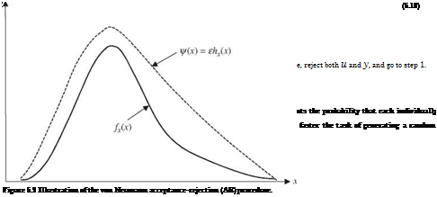
In AR methods, the PDF fx (x) from which a random variate x to be generated is represented, in terms of hx(x), by
fx (x) = ehx (x)g(x) (6.9)
 |
in which є > 1 and 0 < g(x) < 1. Figure 6.2 illustrates the AR method in that the constant є > 1 is chosen such that f (x) = єhx (x) over the sample space of the random variable X. The problem then is to find a function f (x) = єhx(x) such that f (x) > fx(x) and a function hx(x) = f (x)^, from which random variates are generated. The constant є that satisfies f (x) > fx(x) can be obtained from
(see Problem 6.4). Intuitively, the maximum achievable efficiency for an AR method occurs when f (x) = fx(x). In this case, є = 1, g(x) = 1, and the corresponding probability of acceptance P {U < g(Y)} = 1. Therefore, consideration must be given to two aspects when selecting hx(x) for AR methods: (1) the efficiency and exactness of generating a random number from hx(x) and (2) the closeness of hx(x) in imitating fx(x).
Example 6.3 Consider that Manning’s roughness coefficient X of a cast iron pipe is uncertain with a density function fx(x), a < x < b. Develop an AR algorithm using f (x) = c and hx(x) = 1/(b — a), for a < x < b.
1. Generate ui from U(0, 1).
2. Generate U2 from U(0, 1) from which y = a + (b — a)u2.
3. Determine if
 fx [a + (b — a)u2]
c
holds. If yes, accept y; otherwise, reject (U1, y), and return to step 1.
In fact, this is the von Neumann (1951) algorithm for the AR method.
AR methods are important tools for random number generation because they can be very fast in comparison with the CDF-inverse method for distribution models the analytical forms of CDF inverse of which are not available. This approach has been applied to some distributions, such as gamma, resulting in extremely simple and efficient algorithms (Dagpunar, 1988).


Leave a reply