Preventive maintenance

There are two basic categories of maintenance: corrective maintenance and preventive maintenance. Corrective maintenance is performed when the sys­tem experiences in-service failures. Corrective maintenance often involves the needed repair, adjustment, and replacement to restore the failed system back to its normal operating condition. Therefore, corrective maintenance can be regarded as repair, and its stochastic characteristics are describable by the re­pair function, MTTR, and other measures discussed previously in Secs. 5.3.1 through 5.3.3.

On the other hand, preventive maintenance, also called scheduled mainte­nance, is performed in a regular time interval involving periodic inspections,
even if the system is in working condition. In general, preventive maintenance involves not only repair but inspection and some replacements. Preventive maintenance is aimed at postponing failure and prolonging the life of the sys­tem to achieve a longer MTTF for the system. This section will focus on some basic features of preventive maintenance.

From the preceding discussions of what a preventive maintenance program wishes to achieve, it is obvious that preventive maintenance is only a waste of resources for a system having a decreasing or constant hazard function because such an activity cannot decrease the number of failures (see Example 5.7). If the maintenance is neither ideal nor perfect, it may even have an adverse impact on the functionality of the system. Therefore, preventive maintenance is a worthwhile consideration for a system having an increasing hazard function or an aged system (see Problems 5.18 and 5.19).

Ideal maintenance. An ideal maintenance has two features: (1) zero time to com­plete, relatively speaking, as compared with the time interval between mainte­nance, and (2) system is restored to the “as new” condition. The second feature often implies a replacement.

Let tM be the fixed time interval between the scheduled maintenance, and ps, M(t) is the reliability function with preventive maintenance. The reliability of the system at time t, after k preventive maintenances, with ktM < t < (k + 1)tM, for k = 0,1,2,…, is

ps, M(t) = P {no failure in(0, tM], no failure in(tM,2 tM],…,

no failure in((k — 1)tM, ktM], no failure in(ktM, t]}

П no failure in ((i i=1	1)tM, itM], no failure in (ktM, t]
=P

= [ps(tM)]k X ps(t — ktM)

where ps, M(t) is the unmaintained reliability function defined in Eq. (5.1a).

The failure density function with maintenance fM (t) can be obtained from Eq. (5.27), according to Eq. (5.2), as

d [ps, m(t)]
dt

for ktM < t < (k + 1)tM, with k = 0, 1, 2,_______________________ As can be seen from Eqs. (5.27) and

(5.28), the reliability function and failure density function with maintenance in each time segment, defined by two consecutive preventive maintenances, are scaled down by a factor of ps(tM) as compared with the proceeding segment.

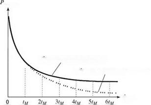With Scheduled Maintenance

Without Scheduled Maintenance

time

Figure 5.12 Reliability function with and without preventive maintenance.

The factor ps(tM) is the fraction of the total components that will survive from one segment of the maintenance period to the next. Geometric illustrations of Eqs. (5.27) and (5.28) are shown in Figs. 5.12 and 5.13, respectively. The envelop curve in Fig. 5.12 (shown by a dashed line) exhibits an exponential decay with a factor of ps(tM).

Similar to an unmaintained system, the hazard function with maintenance can be obtained, according Eq. (5.3), as

hM (t) = Mfor ktM < t < (k + 1)tM, k = 0,1,2,… (5.29)

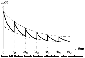Ps, M(t — ktM)

The mean time-to-failure with maintenance MTTFm can be evaluated, ac­cording to Eq. (5.18), as

г ж f-(k+1)tu

MTTFm = / Ps, m (t) dt = ^/ Ps, m (t) dt

•JO k=o ’ k^M

By letting t = t — ktM, the preceding integration for computing the MTTFm can be rewritten as

using 1/(1 — x) = 1 + x + x2 + x3 + x4 + …, for 0 < x < 1.

A preventive maintenance program is worth considering if the reliability with maintenance is greater than the reliability without maintenance. That is,

Letting t = ktM and assuming ps(0) = 1, the preceding expression can be simplified as

Similarly, the implementation of a preventive maintenance program is justifi­able if MTTFm > MTTF or hM(t) > h(t) for all time t.

Example 5.7 Suppose that a system is implemented with preventive maintenance at a regular time interval of tM. The failure density of the system is of an exponential type as

ft(t) = Xe-xt for t > 0

Assuming that the maintenance is ideal, find the expression for the reliability function and the mean time to failure of the system.

Solution The reliability function of the system if no maintenance is in place is (from Table 5.1)

ps(t) = e~lt for t > 0

The reliability of the system under a regular preventive maintenance of time interval tM can be derived, according to Eq. (5.27), as

Ps, M(t) = (e-ltM)k x e-x(t-ktM-1 for ktM < t < (k + 1)tM, k = 0,1,2,…

Ps, M(t) = e lt for t > 0

The mean time to failure of the system with maintenance can be calculated, according to Eq. (5.31), as

As can be seen, with preventive maintenance in place, the reliability function and the mean time to failure of a system having an exponential failure density (constant failure rate) are identical to those without maintenance.

Example 5.8 Consider a system having a uniform failure density bounded in [0, 5 years]. Evaluate the reliability, hazard function, and MTTF for the system if a preventive maintenance program with a 1-year maintenance interval is implemented. Assume that the maintenance is ideal.

Solution The failure density function for the system is

ft(t) = 1/5 for 0 < t < 5

From Table 5.1, the reliability function, hazard function, and MTTF of the system without maintenance, respectively, are

Ps(t) = (5 — t)/5 for 0 < t < 5

h(t) = 1/(t — 5) for 0 < t < 5

and MTTF = 5/2 = 2.5 years

With the maintenance interval tM = 1 year, the reliability function, failure density, hazard function, and the MTTF can be derived, respectively, as

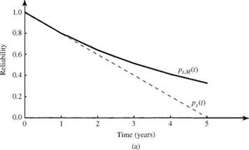
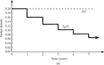
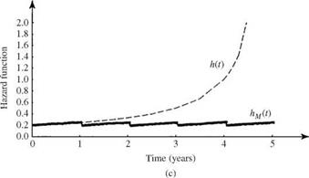
Referring to Fig. 5.6, the hazard function for the system associated with a uniform failure density function is increasing with time. This example shows that the MTTFm is larger than the MTTF, indicating that the scheduled maintenance is beneficial to the system under consideration. Furthermore, plots of the reliability, failure density, and hazard function for this example are shown in Fig. 5.14.

In the context of scheduled maintenance, the number of maintenance ap­plications KM before system failure occurs is a random variable of significant

Figure 5.14 Reliability function (a) with [ps, M(t)] and without [ps(t)] pre­ventive maintenance, failure density function (b) with [ f m(t)] and without [ft(t)] preventive maintenance, and hazard function (c) with [Hm(t)] and without [H(t)] preventive maintenance for Example 5.8.

importance. The probability that the system will undergo exactly k preventive maintenance applications before failure is the probability that system failure occurs before (k + 1)tM, which can be expressed as

qk = [ Ps(tM )]k [1 — Ps(tM)] for k = 0,1,2,… (5.34)

which has the form of a geometric distribution. From Eq. (5.34), the expected number of scheduled maintenance applications before the occurrence of system failure is

and the variance of KM is

ps(tM )[1 + ps(tM )]
[1 — ps(tM)]2

ps(tM )

[1 — ps(tM)]2

The algebraic manipulations used in Eqs. (5.35) and (5.36) employ the following relationships under the condition 0 < x < 1:

Example 5.9 Referring to Example 5.7, having an exponential failure density func­tion, derive the expressions for the expected value and variance of the number of scheduled maintenance applications before the system fails.

Solution According to Eq. (5.35), the expected number of scheduled maintenance ap­plications before failure can be derived as

The variance of the number of scheduled maintenance applications before failure can be derived, according to Eq. (5.36), as

Time variations of the expected value and standard deviation of the number of sched­uled maintenance applications before failure for a system with an exponential failure density function are shown in Fig. 5.15. It is observed clearly that, as expected, when the time interval for scheduled maintenance tM becomes longer relative to the MTTF,

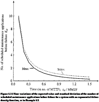the expected number of scheduled maintenance applications E(Km) and its associ­ated standard deviation a ( Km ) decrease. However, the coefficient of variation Q ( Km ) increases. Interestingly, when tM/MTTF = 1, E(Km) = 1/(e — 1) = 0.58, indicat­ing that failure could occur before maintenance if the scheduled maintenance time interval is set to be MTTF under the exponential failure density function.

Example 5.10 Referring to Example 5.8, with a uniform failure density function, compute the expected value and standard deviation of the number of scheduled main­tenance applications before the system fails.

Solution According to Eq. (5.32), the expected number of scheduled maintenance ap­plications before failure can be derived as

The variance of the number of scheduled maintenance applications before failure can be derived, according to Eq. (5.33), as

The standard deviation of the number of scheduled maintenance applications before failure for the system is V20 = 4.47 scheduled maintenance applications.

Imperfect maintenance. Owing to faulty maintenance as a result of human error, the system under repair could fail soon after the preventive maintenance application. If the probability of performing an imperfect maintenance is q, the reliability of the system is to be multiplied by (1 — q) each time maintenance is performed, that is,

Ps, m (t | q) = [(1 — q) ps(tM)]kPs (t — ktM) for ktM < t < (k + 1) M k = 0, 1,2,…

(5.38)

An imperfect maintenance is justifiable only when, at t = ktM,

Example 5.11 Refer to Example 5.7, with an exponential failure density function. Show that implementing an imperfect maintenance is in fact damaging.

Solution By Eq. (5.39), the ratio of reliability functions with and without imperfect maintenance for a system with an exponential failure density is

Ps, m(ktM | q) _ (1 k (e Шм

Ps(ktM) =( q) в-шм

This indicates that performing an imperfect maintenance for a system with an expo­nential failure density function could reduce reliability.

5.3.5 Supportability

For a repairable component, supportability is an issue concerning the ability of the components, when they fail, to receive the required resources for car­rying out the specified maintenance task. It is generally represented by the time to suPPort (TTS), which may include administrative time, logistic time, and mobilization time. Similar to the TTF and TTR, TTS, in reality, also is randomly associated with a probability density function. The cumulative dis­tribution function of the random TTS is called the suPPortability function, rep­resenting the probability that the resources will be available for conducting a repair task at a specified time. Also, other measures of supportability include the mean time to suPPort (MTTS), TTSP, and suPPort success, similar to those defined for maintainability, with the repair density function replaced by the density function of the TTS.