Poisson distribution
The Poisson distribution has the PMF as
e — vV x
px(x | v) =—;— for x = 0,1,2,… (2.53)
x!
where the parameter v > 0 represents the mean of a Poisson random variable. Unlike the binomial random variables, Poisson random variables have no upper bound. A recursive formula for calculating the Poisson PMF is (Drane et al., 1993)
Px (x | v) = (X) Px (x — 11 v) = Rp (x) Px (x — 11 v) for x = 1,2,… (2.54)
with px(x = 0 | v) = e—v and RP (x) = v/x. When v and p ^ 0 while np = v = constant, the term RB (x) in Eq. (2.52) for the binomial distribution becomes RP (x) for the Poisson distribution. Tietjen (1994) presents a simple recursive scheme for computing the Poisson cumulative probability.
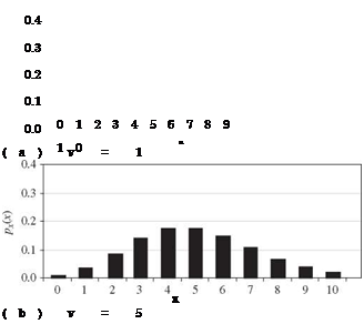
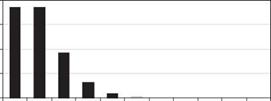
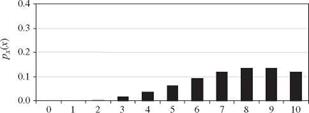
For a Poisson random variable, the mean and the variance are identical to v. Plots of Poisson PMFs corresponding to different values of v are shown in Fig. 2.17. As shown in Fig. 2.15, Poisson random variables also have the same reproductive property as binomial random variables. That is, the sum of several independent Poisson random variables, each with a parameter vk, is still a Poisson random variable with a parameter v1 + v2 + ■ ■ ■ + vK. The skewness
 |
|
|

coefficient of a Poisson random variable is 1Д/ЇЇ, indicating that the shape of the distribution approaches symmetry as v gets large.
The Poisson distribution has been applied widely in modeling the number of occurrences of a random event within a specified time or space interval. Equation (2.2) can be modified as
p-lt ( W )X
Px (x | X, t) = for x = 0,1,2,… (2.55)
X!
in which the parameter X can be interpreted as the average rate of occurrence of the random event in a time interval (0, t).
Example 2.15 Referring to Example 2.14, the use of binomial distribution assumes, implicitly, that the overtopping occurs, at most, once each year. The probability is zero for having more than two overtopping events annually. Relax this assumption and use the Poisson distribution to reevaluate the probability of overtopping during a 100-year period.
Solution Using the Poisson distribution, one has to determine the average number of overtopping events in a period of 100 years. For a 50-year event, the average rate of overtopping is X = 0.02/year. Therefore, the average number of overtopping events in a period of 100 years can be obtained as v = (0.02)( 100) = 2 overtoppings. The probability of overtopping in an 100-year period, using a Poisson distribution, is
P (overtopping occurs in a 100-year period)
= P (overtopping occurs at least once in a 100-year period)
= 1 — P (no overtopping occurs in a 100-year period)
= 1 — p(X = 0 | v = 2) = 1 — e—2 = 1 — 0.1353 = 0.8647
Comparing with the result from Example 2.14, use of the Poisson distribution results in a slightly smaller risk of overtopping.
To relax the restriction of equality of the mean and variance for the Poisson distribution, Consul and Jain (1973) introduced the generalized Poisson distribution (GPD) having two parameters в and X with the probability mass function as
в(в I xX)n 1e (e +xX)
px(x | в, X) = for x = 0,1,2,…; X > 0 (2.56)
x!
The parameters (в, X) can be determined by the first two moments (Consul, 1989) as
вв
E(X)=1—X Var(X)=(T-D3 e.57)
The variance of the GPD model can be greater than, equal to, or less than the mean depending on whether the second parameter X is positive, zero, or negative. The values of the mean and variance of a GPD random variable tend to increase as в increases. The GPD model has greater flexibility to fit various types of random counting processes, such as binomial, negative binomial, or Poisson, and many other observed data.


Leave a reply