Category Hydrosystems Engineering Reliability Assessment and Risk Analysis

Some Continuous Univariate Probability Distributions

Several continuous PDFs are used frequently in reliability analysis. They in­clude normal, lognormal, gamma, Weibull, and exponential distributions. Other distributions, such as beta and extremal distributions, also are used sometimes.

The relations among the various continuous distributions considered in this chapter and others are shown in Fig. 2.15.

1.6.1 Normal (Gaussian) distribution

The normal distribution is a well-known probability distribution involving two parameters: the mean and variance. A normal random variable having the mean /гх and variance a2 is denoted herein as X ~ N (tx, ax) with the PDF

Подпись: 2Подпись: 1 {x Hx 2 V ax Подпись: for —TO < x < TO (2.58)fN (x | tx, ax2) = —І— exp ■sj2n ax

The relationship between tx and ax and the L-moments are tx = Л1 and

ax = рЯ^2.

The normal distribution is bell-shaped and symmetric with respect to the mean [ix. Therefore, the skewness coefficient of a normal random variable is zero. Owing to the symmetry of the PDF, all odd-order central moments are zero. Thekurtosis of a normal random variable is kx = 3.0. Referring to Fig. 2.15, a lin­ear function of several normal random variables also is normal. That is, the lin­ear combination of K normal random variables W = a1 X1 + a2X2 + ■ ■ ■ + aKXK, with Xk ~ N(tk, ak), for k = 1, 2,…, K, is also a normal random variable with the mean tw and variance aW, respectively, as

K K K-1 K

t^w У ^ akt^k aw У ^ akak + 2 У ^ У ^ akakCov(Xk, Xk)

k = 1 k = 1 k = 1 k = k+1

The normal distribution sometimes provides a viable alternative to approx­imate the probability of a nonnormal random variable. Of course, the accu­racy of such an approximation depends on how closely the distribution of the nonnormal random variable resembles the normal distribution. An important theorem relating to the sum of independent random variables is the central limit theorem, which loosely states that the distribution of the sum of a number of independent random variables, regardless of their individual distributions, can be approximated by a normal distribution, as long as none of the vari­ables has a dominant effect on the sum. The larger the number of random variables involved in the summation, the better is the approximation. Because many natural processes can be thought of as the summation of a large number of independent component processes, none dominating the others, the normal distribution is a reasonable approximation for these overall processes. Finally, Dowson and Wragg (1973) have shown that when only the mean and variance are specified, the maximum entropy distribution on the interval (-to, +to) is the normal distribution. That is, when only the first two moments are specified, the use of the normal distribution implies more information about the nature of the underlying process specified than any other distributions.

Probability computations for normal random variables are made by first transforming the original variable to a standardized normal variable Z by

Eq. (2.49), that is,


Z = (X — /лх )/ax

Подпись: Ф (z) Подпись: 1 — exp л/2Л Подпись: z2 2 Подпись: for — TO < z < TO Подпись: (2.59)

in which Z has a mean of zero and a variance of one. Since Z is a linear function of the normal random variable X, Z is therefore normally distributed, that is, Z ~ N(jaz = 0, az = 1). The PDF of Z, called the standard normal distribution, can be obtained easily as

Some Continuous Univariate Probability Distributions Some Continuous Univariate Probability Distributions

The general expressions for the product-moments of the standard normal ran­dom variable are

where z = (x — их)/aX, and Ф^) is the standard normal CDF defined as

Подпись: (2.62)Ф( z) = ф (z) dz

— TO

Figure 2.18 shows the shape of the PDF of the standard normal random variable.
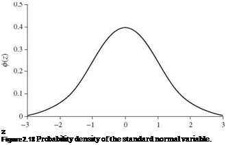
Подпись: z Figure 2.18 Probability density of the standard normal variable.

The integral result of Eq. (2.62) is not analytically available. A table of the standard normal CDF, such as Table 2.2 or similar, can be found in many statistics textbooks (Abramowitz and Stegun, 1972; Haan, 1977; Blank, 1980;

TABLE 2.2 Table of Standard Normal Probability, Ф( z) = P(Z < z)

z

0.00

0.01

0.02

0.03

0.04

0.05

0.06

0.07

0.08

0.09

0.0

0.5000

0.5040

0.5080

0.5120

0.5160

0.5199

0.5239

0.5279

0.5319

0.5359

0.1

0.5398

0.5438

0.5478

0.5517

0.5557

0.5596

0.5636

0.5675

0.5714

0.5753

0.2

0.5793

0.5832

0.5871

0.5910

0.5948

0.5987

0.6026

0.6064

0.6103

0.6141

0.3

0.6179

0.6217

0.6255

0.6293

0.6331

0.6368

0.6406

0.6443

0.6480

0.6517

0.4

0.6554

0.6591

0.6628

0.6664

0.6700

0.6736

0.6772

0.6808

0.6844

0.6879

0.5

0.6915

0.6950

0.6985

0.7019

0.7054

0.7088

0.7123

0.7157

0.7190

0.7224

0.6

0.7257

0.7291

0.7324

0.7357

0.7389

0.7422

0.7454

0.7486

0.7517

0.7549

0.7

0.7580

0.7611

0.7642

0.7673

0.7704

0.7734

0.7764

0.7794

0.7823

0.7852

0.8

0.7881

0.7910

0.7939

0.7967

0.7995

0.8023

0.8051

0.8078

0.8106

0.8133

0.9

0.8159

0.8186

0.8212

0.8238

0.8264

0.8289

0.8315

0.8340

0.8365

0.8389

1.0

0.8413

0.8438

0.8461

0.8485

0.8508

0.8531

0.8554

0.8577

0.8599

0.8621

1.1

0.8643

0.8665

0.8686

0.8708

0.8729

0.8749

0.8770

0.8790

0.8810

0.8830

1.2

0.8849

0.8869

0.8888

0.8907

0.8925

0.8944

0.8962

0.8980

0.8997

0.9015

1.3

0.9032

0.9049

0.9066

0.9082

0.9099

0.9115

0.9131

0.9147

0.9162

0.9177

1.4

0.9192

0.9207

0.9222

0.9236

0.9251

0.9265

0.9279

0.9292

0.9306

0.9319

1.5

0.9332

0.9345

0.9357

0.9370

0.9382

0.9394

0.9406

0.9418

0.9429

0.9441

1.6

0.9452

0.9463

0.9474

0.9484

0.9495

0.9505

0.9515

0.9525

0.9535

0.9545

1.7

0.9554

0.9564

0.9573

0.9582

0.9591

0.9599

0.9608

0.9616

0.9625

0.9633

1.8

0.9641

0.9649

0.9656

0.9664

0.9671

0.9678

0.9686

0.9693

0.9699

0.9706

1.9

0.9713

0.9719

0.9726

0.9732

0.9738

0.9744

0.9750

0.9756

0.9761

0.9767

2.0

0.9772

0.9778

0.9783

0.9788

0.9793

0.9798

0.9803

0.9808

0.9812

0.9817

2.1

0.9821

0.9826

0.9830

0.9834

0.9838

0.9842

0.9846

0.9850

0.9854

0.9857

2.2

0.9861

0.9864

0.9868

0.9871

0.9875

0.9878

0.9881

0.9884

0.9887

0.9890

2.3

0.9893

0.9896

0.9898

0.9901

0.9904

0.9906

0.9909

0.9911

0.9913

0.9916

2.4

0.9918

0.9920

0.9922

0.9925

0.9927

0.9929

0.9931

0.9932

0.9934

0.9936

2.5

0.9938

0.9940

0.9941

0.9943

0.9945

0.9946

0.9948

0.9949

0.9951

0.9952

2.6

0.9953

0.9955

0.9956

0.9957

0.9959

0.9960

0.9961

0.9962

0.9963

0.9964

2.7

0.9965

0.9966

0.9967

0.9968

0.9969

0.9970

0.9971

0.9972

0.9973

0.9974

2.8

0.9974

0.9975

0.9976

0.9977

0.9977

0.9978

0.9979

0.9979

0.9980

0.9981

2.9

0.9981

0.9982

0.9982

0.9983

0.9984

0.9984

0.9985

0.9985

0.9986

0.9986

3.0

0.9987

0.9987

0.9987

0.9988

0.9988

0.9989

0.9989

0.9989

0.9990

0.9990

3.1

0.9990

0.9991

0.9991

0.9991

0.9992

0.9992

0.9992

0.9992

0.9993

0.9993

3.2

0.9993

0.9993

0.9994

0.9994

0.9994

0.9994

0.9994

0.9995

0.9995

0.9995

3.3

0.9995

0.9995

0.9995

0.9996

0.9996

0.9996

0.9996

0.9996

0.9996

0.9997

3.4

0.9997

0.9997

0.9997

0.9997

0.9997

0.9997

0.9997

0.9997

0.9997

0.9998

NOTE: Ф(-г) = 1 – Ф(г), z > 0.

Devore, 1987). For numerical computation purposes, several highly accurate approximations are available for determining Ф(z). One such approximation is the polynomial approximation (Abramowitz and Stegun, 1972)

Ф(z) = 1 – ф(z)(b1t + b2t2 + b3t3 + b4t4 + b5t5) for z > 0 (2.63)

in which t = 1/(1 + 0.2316419z), b1 = 0.31938153, b2 = -0.356563782, b3 = 1.781477937, b4 = -1.821255978, and b5 = 1.33027443. The maximum absolute error of the approximation is 7.5 x 10⁻⁸, which is sufficiently accurate for most practical applications. Note that Eq. (2.63) is applicable to the non-negative­valued z. For z < 0, the value of standard normal CDF can be computed as ФЫ = 1 – Ф(|z|) by the symmetry of ф(z). Approximation equations, such as

Eq. (2.63), can be programmed easily for probability computations without needing the table of the standard normal CDF.

Some Continuous Univariate Probability Distributions Подпись: for 0.5 < p < 1 Подпись: (2.64)

Equally practical is the inverse operation of finding the standard normal quantile zp with the specified probability level p. The standard normal CDF table can be used, along with some mechanism of interpolation, to determine zp. However, for practical algebraic computations with a computer, the following rational approximation can be used (Abramowitz and Stegun, 1972):

in which p = ), t = y/-2 ln(1 – p), c0 = 2.515517, ci = 0.802853, c2 =

0.010328, d1 = 1.432788, d2 = 0.189269, and d3 = 0.001308. The correspond­ing maximum absolute error by this rational approximation is 4.5 x 10⁻⁴. Note that Eq. (2.64) is valid for the value of Ф^) that lies between [0.5, 1]. When p < 0.5, one can still use Eq. (2.64) by letting t = J-2 x ln(p) and attaching a negative sign to the computed quantile value. Vedder (1995) proposed a sim­ple approximation for computing the standard normal cumulative probabilities and standard normal quantiles.

Example 2.16 Referring to Example 2.14, determine the probability of more than five overtopping events over a 100-year period using a normal approximation.

Solution In this problem, the random variable X of interest is the number of over­topping events in a 100-year period. The exact distribution of X is binomial with parameters n = 100 and p = 0.02 or the Poisson distribution with a parameter v = 2. The exact probability of having more than five occurrences of overtopping in 100 years can be computed as

Подпись: P (X > 6) =Подпись:Подпись:Some Continuous Univariate Probability Distributions

Подпись: = 1 - P (X < Подпись: 100 x Подпись: (0.02)x (0.98)100-x Подпись: x = 6

P(X > 5) =

= 1 – 0.9845 = 0.0155

As can be seen, there are a total of six terms to be summed up on the right-hand side. Although the computation of probability by hand is within the realm of a reasonable task, the following approximation is viable. Using a normal probability approxima­tion, the mean and variance of X are

/Px = np = (100)(0.02) = 2.0 al = npq = (100)(0.02)(0.98) = 1.96

The preceding binomial probability can be approximated as

P(X > 6) ^ P(X > 5.5) = 1 – P(X < 5.5) = 1 – P [Z < (5.5 – 2.0)/УЇ96]

= 1 – Ф(2.5) = 1 – 0.9938 = 0.062

DeGroot (1975) showed that when np 1.5 >

1.07, the error of using the normal dis­tribution to approximate the binomial probability did not exceed 0.05. The error in the approximation gets smaller as the value of np15 becomes larger. For this exam­ple, np15 = 0.283 < 1.07, and the accuracy of approximation was not satisfactory as shown.

Example 2.17 (adopted from Mays and Tung, 1992) The annual maximum flood magnitude in a river has a normal distribution with a mean of 6000 ft3/s and standard deviation of 4000 ft3/s. (a) What is the annual probability that the flood magnitude would exceed 10,000 ft3/s? (b) Determine the flood magnitude with a return period of 100 years.

Solution (a) Let Q be the random annual maximum flood magnitude. Since Q has a nor­mal distribution with a mean xq = 6000 ft3/s and standard deviation oq = 4000 ft3/s, the probability of the annual maximum flood magnitude exceeding 10,000 ft3/s is

P(Q > 10, 000) = 1 – P [Z < (10, 000 – 6000)/4000]

= 1 – Ф(1.00) = 1 – 0.8413 = 0.1587

(b) A flood event with a 100-year return period represents the event the magnitude of which has, on average, an annual probability of 0.01 being exceeded. That is, P(Q > 7100) = 0.01, in which 7100 is the magnitude of the 100-year flood. This part of the problem is to determine 7100 from

P(Q < 7100) = 1 – P(Q > 7100) = 0.99

because P(Q < 7100) = P {Z < [(7100 – xq)/oq]}

= P [Z < (7100 – 6000)/4000]

= Ф[71.00 – 6000)/4000] = 0.99

From Table 2.2 or Eq. (2.64), one can find that Ф(2.33) = 0.99. Therefore,

(7100 – 6000)/4000 = 2.33

which gives that the magnitude of the 100-year flood event as 7100 = 15, 320 ft3/s.

Poisson distribution

The Poisson distribution has the PMF as

e — vV x

px(x | v) =—;— for x = 0,1,2,… (2.53)

x!

where the parameter v > 0 represents the mean of a Poisson random variable. Unlike the binomial random variables, Poisson random variables have no upper bound. A recursive formula for calculating the Poisson PMF is (Drane et al., 1993)

Px (x | v) = (X) Px (x — 11 v) = Rp (x) Px (x — 11 v) for x = 1,2,… (2.54)

with px(x = 0 | v) = e—v and RP (x) = v/x. When v and p ^ 0 while np = v = constant, the term RB (x) in Eq. (2.52) for the binomial distribution becomes RP (x) for the Poisson distribution. Tietjen (1994) presents a simple recursive scheme for computing the Poisson cumulative probability.

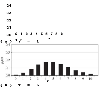
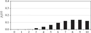
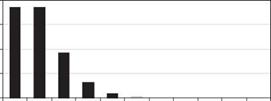
For a Poisson random variable, the mean and the variance are identical to v. Plots of Poisson PMFs corresponding to different values of v are shown in Fig. 2.17. As shown in Fig. 2.15, Poisson random variables also have the same re­productive property as binomial random variables. That is, the sum of several independent Poisson random variables, each with a parameter vk, is still a Poisson random variable with a parameter v1 + v2 + ■ ■ ■ + vK. The skewness

Poisson distribution

Poisson distribution

x

(c) v = 9

Figure 2.17 Probability mass functions of Poisson random variables with different parameter values.


Poisson distribution

coefficient of a Poisson random variable is 1Д/ЇЇ, indicating that the shape of the distribution approaches symmetry as v gets large.

The Poisson distribution has been applied widely in modeling the number of occurrences of a random event within a specified time or space interval. Equation (2.2) can be modified as

p-lt ( W )X

Px (x | X, t) = for x = 0,1,2,… (2.55)

X!

in which the parameter X can be interpreted as the average rate of occurrence of the random event in a time interval (0, t).

Example 2.15 Referring to Example 2.14, the use of binomial distribution assumes, implicitly, that the overtopping occurs, at most, once each year. The probability is zero for having more than two overtopping events annually. Relax this assumption and use the Poisson distribution to reevaluate the probability of overtopping during a 100-year period.

Solution Using the Poisson distribution, one has to determine the average number of overtopping events in a period of 100 years. For a 50-year event, the average rate of overtopping is X = 0.02/year. Therefore, the average number of overtopping events in a period of 100 years can be obtained as v = (0.02)( 100) = 2 overtoppings. The probability of overtopping in an 100-year period, using a Poisson distribution, is

P (overtopping occurs in a 100-year period)

= P (overtopping occurs at least once in a 100-year period)

= 1 — P (no overtopping occurs in a 100-year period)

= 1 — p(X = 0 | v = 2) = 1 — e—2 = 1 — 0.1353 = 0.8647

Comparing with the result from Example 2.14, use of the Poisson distribution results in a slightly smaller risk of overtopping.

To relax the restriction of equality of the mean and variance for the Pois­son distribution, Consul and Jain (1973) introduced the generalized Poisson distribution (GPD) having two parameters в and X with the probability mass function as

в(в I xX)n 1e (e +xX)

px(x | в, X) = for x = 0,1,2,…; X > 0 (2.56)

x!

The parameters (в, X) can be determined by the first two moments (Consul, 1989) as

вв

E(X)=1—X Var(X)=(T-D3 e.57)

The variance of the GPD model can be greater than, equal to, or less than the mean depending on whether the second parameter X is positive, zero, or negative. The values of the mean and variance of a GPD random variable tend to increase as в increases. The GPD model has greater flexibility to fit various types of random counting processes, such as binomial, negative binomial, or Poisson, and many other observed data.

Binomial distribution

The binomial distribution is applicable to random processes with only two types of outcomes. The state of components or subsystems in many hydrosystems can be classified as either functioning or failed, which is a typical example of a binary outcome. Consider an experiment involving a total of n independent trials with each trial having two possible outcomes, say, success or failure. In each trial, if the probability of having a successful outcome is p, the probability of having x successes in n trials can be computed as

Px(x) = Cn, xpxqn-x for x = 0,1,2,…,n (2.51)

where Cn, x is the binomial coefficient, and q = 1 – p, the probability of having a failure in each trial. Computationally, it is convenient to use the following recursive formula for evaluating the binomial PMF (Drane et al., 1993):

Px(x | n, p) = (——————- x——– JVqjPx(x — 11 n, p) = Rb(x)Px(x — 11 n, p) (2.52)

for x = 0, 1,2,…, n, with the initial probability px(x = 0|n, p) = qn. A simple recursive scheme for computing the binomial cumulative probability is given by Tietjen (1994).

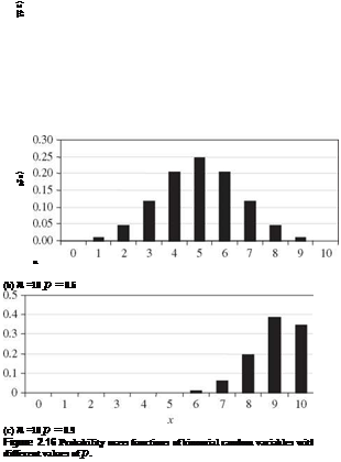
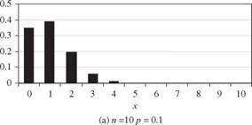
A random variable X having a binomial distribution with parameters n and p has the expectation E (X) = np and variance Var(X) = npq. Shape of the PMF of a binomial random variable depends on the values of p and q. The skewness coefficient of a binomial random variable is (q — p)/^/npq. Hence the PMF is positively skewed if p <q, symmetric if p = q = 0.5, and negatively skewed if p > q. Plots of binomial PMFs for different values of p with a fixed n are shown in Fig. 2.16. Referring to Fig. 2.15, the sum of several independent binomial random variables, each with a common parameter p and different nk s, is still a binomial random variable with parameters p and £knk.

Example 2.14 A roadway-crossing structure, such as a bridge or a box or pipe cul­vert, is designed to pass a flood with a return period of 50 years. In other words, the annual probability that the roadway-crossing structure would be overtopped is a 1-in-50 chance or 1/50 = 0.02. What is the probability that the structure would be overtopped over an expected service life of 100 years?

Solution In this example, the random variable X is the number of times the roadway­crossing structure will be overtopped over a 100-year period. One can treat each year as an independent trial from which the roadway structure could be overtopped or not overtopped. Since the outcome of each “trial” is binary, the binomial distribution is applicable.

Binomial distribution

Binomial distribution

Binomial distribution

The event of interest is the overtopping of the roadway structure. The probability of such an event occurring in each trial (namely, each year), is 0.02. A period of 100 years represents 100 trials. Hence, in the binomial distribution model, the parameters are p = 0.02 and n = 100. The probability that overtopping occurs in a period of 100 years can be calculated, according to Eq. (2.51), as

P (overtopping occurs in an 100-year period)

= P (overtopping occurs at least once in an 100-year period)

= P(X > 11 n = 100, p = 0.02)

100 100

= X) Px(x) = X) C1°°>x(0.02)x(0.98)100-x

x = 1 x = 1

This equation for computing the overtopping probability requires evaluations of 100 binomial terms, which could be very cumbersome. In this case, one could solve the problem by looking at the other side of the coin, i. e., the nonoccurrence of overtopping events. In other words,

P (overtopping occurs in a 100-year period)

= P (overtopping occurs at least once in a 100-year period)

= 1 — P (no overtopping occurs in a 100-year period)

= 1 — p( X = 0) = 1 — (0.98)100

= 1 — 0.1326 = 0.8674

Calculation of the overtopping risk, as illustrated in this example, is made under an implicit assumption that the occurrence of floods is a stationary process. In other words, the flood-producing random mechanism for the watershed under considera­tion does not change with time. For a watershed undergoing changes in hydrologic characteristics, one should be cautious about the estimated risk.

The preceding example illustrates the basic application of the binomial dis­tribution to reliability analysis. A commonly used alternative is the Poisson distribution described in the next section. More detailed descriptions of these two distributions in time-dependent reliability analysis of hydrosystems infras­tructural engineering are given in Sec. 4.7.

Discrete Univariate Probability Distributions

In the reliability analysis of hydrosystems engineering problems, several proba­bility distributions are used frequently. Based on the nature of the random vari­able, probability distributions are classified into discrete and continuous types. In this section, two discrete distributions, namely, the binomial distribution and the Poisson distribution, that are used commonly in hydrosystems reliability analysis, are described. Section 2.6 describes several frequently used univari­ate continuous distributions. For the distributions discussed in this chapter and others not included herein, their relationships are shown in Fig. 2.15.

Discrete Univariate Probability Distributions

Figure 2.15 Relationships among univariate distributions. (After Leemis, 1986.)

Computations of probability and quantiles for the great majority of the dis­tribution functions described in Secs. 2.5 and 2.6 are available in Microsoft Excel.

Covariance and correlation coefficient

When a problem involves two dependent random variables, the degree of linear dependence between the two can be measured by the correlation coefficient pXyy, which is defined as

Corr(X, Y) = px, y = Cov(X, Y )laTay (2.47)

where Cov(X, Y) is the covariance between random variables X and Y, defined as

Cov(X, Y) = E[(X – ,ix)(Y – iiy)] = E(XY) – pPy (2.48)

Various types of correlation coefficients have been developed in statistics for measuring the degree of association between random variables. The one defined by Eq. (2.47) is called the Pearson product-moment correlation coefficient, or correlation coefficient for short in this and general use.

It can be shown easily that Cov(X^, X’2) = Corr(Xь X2), with X^ and X’2 being the standardized random variables. In probability and statistics, a random variable can be standardized as

X’ = (X – px)/ax (2.49)

Hence a standardized random variable has zero mean and unit variance. Stan­dardization will not affect the skewness coefficient and kurtosis of a random variable because they are dimensionless.

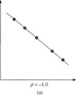
Figure 2.14 graphically illustrates several cases of the correlation coeffi­cient. If the two random variables X and Y are statistically independent, then Corr(X, Y) = Cov(X, Y) = 0 (Fig. 2.14c). However, the reverse statement is not necessarily true, as shown in Fig. 2.14d. If the random variables involved are not statistically independent, Eq. (2.70) for computing the variance of the sum of several random variables can be generalized as

/ k K K-1 K

Var ]T akXk = ]T aal + 2 £ ]T akak, Cov(Xk, X„) (2.50)

k = 1 ) k = 1 k = 1 k=k+1

Example 2.12 (after Tung and Yen, 2005) Perhaps the assumption of independence of Pm, Im, and Em in Example 2.11 may not be reasonable in reality. One examines the historical data closely and finds that correlations exist among the three hydrologic random variables. Analysis of data reveals that Corr(Pm, Im) = 0.8, Corr(Pm, Em) = -0.4, and Corr(Im, Em) = – 0.3. Recalculate the standard deviation associated with the end-of-month storage volume.

y


y


Подпись: XCovariance and correlation coefficient• •

_ • • • . •

• • •

p = 0.8

Подпись: X

(b)

У


У


x


x


p = 0.0

(c)


p = 0.0

(d)


Covariance and correlation coefficient

Covariance and correlation coefficient

Figure 2.14 Different cases of correlation between two random variables:

(a) perfectly linearly correlated in opposite directions; (b) strongly linearly correlated in a positive direction; (c) uncorrelated in linear fashion; (d) per­fectly correlated in nonlinear fashion but uncorrelated linearly.

Solution By Eq. (2.50), the variance of the reservoir storage volume at the end of the month can be calculated as

Var(Sm+1) = ar (Pm) + Var(Im) + Var(Em) + 2 Cov(Pm, Im)

— 2 Cov(Pm, Em) — 2 Cov(Im, Em)

= Var(Pm) + Var(Im) + Var(Em) + 2 Corr(Pm, Im)o(Pm)o(Im)

— 2Corr(Pm, Em)&(Pm)&(Em) — 2 Corr(Im, Em)&(Im)&(Em) = (500)2 + (2000)2 + (1000)2 + 2(0.8)(500)(2000)

— 2(—0.4)(500)(1000) — 2(—0.3)(2000)(1000)

= 8.45(1000 m3)2

The corresponding standard deviation of the end-of-month storage volume is a(Sm+1) = V845 x 1000 = 2910 m3

In this case, consideration of correlation increases the standard deviation by 27 percent compared with the uncorrelated case in Example 2.11.

Example 2.13 Referring to Example 2.7, compute correlation coefficient between X and Y.

Solution Referring to Eqs. (2.47) and (2.48), computation of the correlation coefficient requires the determination of xx, xy, ax, and ay from the marginal PDFs of X and Y:

4 -t – 3×2 4 -t – 3 y2

fx(x) = ——— for 0 < x < 2 fy(y) = ——— for 0 < y < 2

as well as E(XY) from their joint PDF obtained earlier:

Подпись: fx,y(x, y) = ■Подпись:3( x2 + y2)

32

Covariance and correlation coefficient

From the marginal PDFs, the first two moments of X and Y about the origin can be obtained easily as

Var(X) = E(X2) – (Mx)2 = 73/240 = Var(Y)

To calculate Cov(X, Y), one could first compute E(XY) from the joint PDF as

E(XY) = f ( xyfx, y(x, y) dxdy = |

J0 J0

Covariance and correlation coefficient

Then the covariance of X and Y, according to Eq. (2.48), is Cov(X, Y) = E (XY) – nxny = -1/16 The correlation between X and Y can be obtained as

Skewness coefficient and kurtosis

The asymmetry of the PDF of a random variable is measured by the skewness coefficient Yx, defined as

Skewness coefficient and kurtosis

E [(X – ,x)3]


_ _M3_ Yx = ,,1.5 ^2


(2.40)


a


Skewness coefficient and kurtosis
The skewness coefficient is dimensionless and is related to the third-order central moment. The sign of the skewness coefficient indicates the degree of symmetry of the probability distribution function. If yx = 0, the distribution is symmetric about its mean. When yx > 0, the distribution has a long tail to the right, whereas yx < 0 indicates that the distribution has a long tail to the left. Shapes of distribution functions with different values of skewness coeffi­cients and the relative positions of the mean, median, and mode are shown in Fig. 2.13.

Similarly, the degree of asymmetry can be measured by the L-skewness coefficient t3, defined as

тз = A.3/A.2 (2.41)

The value of the L-skewness coefficient for all feasible distribution functions must lie within the interval of [-1, 1] (Hosking, 1986).

Another indicator of the asymmetry is the Pearson skewness coefficient, defined as

Подпись:l^x xmo

Y1 =————-

®x

As can be seen, the Pearson skewness coefficient does not require computing the third-order moment. In practice, product-moments higher than the third order are used less because they are unreliable and inaccurate when estimated from a small number of samples. Equations used to compute the sample product – moments are listed in the last column of Table 2.1.

Skewness coefficient and kurtosis Подпись: E [(X - ілх)4] Подпись: (2.43)

Kurtosis kx is a measure of the peakedness of a distribution. It is related to the fourth-order central moment of a random variable as

with kx > 0. For a random variable having a normal distribution (Sec. 2.6.1), its kurtosis is equal to 3. Sometimes the coefficient of excess, defined as ex = kx — 3, is used. For all feasible distribution functions, the skewness coefficient and kurtosis must satisfy the following inequality relationship (Stuart and Ord,

1987)

Подпись: (2.44)Подпись: (2.45)yX + 1 < Kx

By the definition of L-moments, the L-kurtosis is defined as

T4 = Л4/Л2

Skewness coefficient and kurtosis Подпись: (2.46)

Similarly, the relationship between the L-skewness and L-kurtosis for all fea­sible probability distribution functions must satisfy (Hosking, 1986)

Royston (1992) conducted an analysis comparing the performance of sample skewness and kurtosis defined by the product-moments and L-moments. Results indicated that the L-skewness and L-kurtosis have clear advantages

over the conventional product-moments in terms of being easy to interpret, fairly robust to outliers, and less unbiased in small samples.

Variance, standard deviation, and coefficient of variation

The spreading of a random variable over its range is measured by the variance, which is defined for the continuous case as

/

TO

(X – fZx)2 fx(x) dx (2.36)

-TO

The variance is the second-order central moment. The positive square root of the variance is called the standard deviation ax, which is often used as a measure of the degree of uncertainty associated with a random variable.

The standard deviation has the same units as the random variable. To com­pare the degree of uncertainty of two random variables with different units, a dimensionless measure ^x = ax/^x, called the coefficient of variation, is useful. By its definition, the coefficient of variation indicates the variation of a random variable relative to its mean. Similar to the standard deviation, the second- order L-moment Л2 is a measure of dispersion of a random variable. The ratio of Л2 to Л1, that is, t2 = k2/k1, is called the L-coefficient of variation.

Three important properties of the variance are

1. Var(a) = 0 when a is a constant. (2.37)

2. Var(X) = E(X2) – E2(X) = ^ – ii2x (2.38)

3. The variance of the sum of several independent random variables equal the sum of variance of the individual random variables, that is,

Var f Y akXЛ = Y a (2.39)

k = 1 ) k = 1

where ak is a constant, and ak is the standard deviation of random variable Xk, k = 1,2,…, K.

Variance, standard deviation, and coefficient of variation

Example 2.11 (modified from Mays and Tung, 1992) Consider the mass balance of a surface reservoir over a 1-month period. The end-of-month storage S can be computed as

in which the subscript m is an indicator for month, Sm is the initial storage volume in the reservoir, Pm is the precipitation amount on the reservoir surface, Im is the surface-runoff inflow, Em is the total monthly evaporation amount from the reservoir surface, and Tm is the controlled monthly release volume from the reservoir.

It is assumed that at the beginning of the month, the initial storage volume and total monthly release are known. The monthly total precipitation amount, surface-runoff inflow, and evaporation are uncertain and are assumed to be independent random variables. The means and standard deviations of Pm, Im, and Em from historical data for month m are estimated as

E (Pm) = 1000 m3, E (Im) = 8000 m3, E (Em) = 3000 m3 a (Pm) = 500 m3, a (Im) = 2000 m3, a (Em) = 1000 m3

Determine the mean and standard deviation of the storage volume in the reservoir by the end of the month if the initial storage volume is 20,000 m3 and the designated release for the month is 10,000 m3.

Solution From Eq. (2.31), the mean of the end-of-month storage volume in the reservoir can be determined as

E ( Sm+1) = Sm + E ( Pm) + E (Im) – E ( Em) — Tm

= 20, 000 + 1000 + 8000 – 3000 – 10, 000 = 16, 000 m3

Since the random hydrologic variables are statistically independent, the variance of the end-of-month storage volume in the reservoir can be obtained, from Eq. (2.39), as

Var( Sm+1) = Var( Pm) + Var( Im) + Var( Em)

= [(0.5)2 + (2)2 + (1)2] x (1000m3)2 = 5.25 x (1000m3)2

The standard deviation and coefficient of variation of Sm+1 then are

a(Sm+1) = V525 x 1000 = 2290m3 and Q(Sm+1) = 2290/16,000 = 0.143

Mean, mode, median, and quantiles

Подпись:Подпись: (2.30)

Mean, mode, median, and quantiles Mean, mode, median, and quantiles Подпись: [1 — Fx (x)] dx

The central tendency of a continuous random variable X is commonly repre­sented by its expectation, which is the first-order moment about the origin:

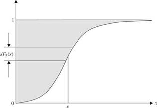
This expectation is also known as the mean of a random variable. It can be seen easily that the mean of a random variable is the first-order L-moment Л1. Geometrically, the mean or expectation of a random variable is the location of the centroid of the PDF or PMF. The second and third integrations in Eq. (2.30) indicate that the mean of a random variable is the shaded area shown in Fig. 2.11.

The following two operational properties of the expectation are useful:

1. The expectation of the sum of several random variables (regardless of their dependence) equals the sum of the expectation of the individual random

Fx(x)

Mean, mode, median, and quantiles

Figure 2.11 Geometric interpretation of the mean.


variable, that is,

Подпись: (2.31)( K K E akXk = ^2 akMk

k = і k = і

in which pk = E(Xk), for k = 1,2,…, K.

2. The expectation of multiplication of several independent random variables equals the product of the expectation of the individual random variables, that is,

E П Xk = П Mk (2.32)

k = 1 k = 1

Подпись: Fx (xmd) Подпись: •^md fx(x) dx = 0.5 — TO Подпись: (2.33)

Two other types of measures of central tendency of a random variable, namely, the median and mode, are sometimes used in practice. The median of a ran­dom variable is the value that splits the distribution into two equal halves. Mathematically, the median xmd of a continuous random variable satisfies

The median, therefore, is the 50th quantile (or percentile) of random variable X. In general, the 100pth quantile of a random variable X is a quantity xp that satisfies

P (X < xp) = Fx(xp) = p (2.34)

The mode is the value of a random variable at which the value of a PDF is peaked. The mode xmo of a random variable X can be obtained by solving the

Подпись: dfx(X) д X Подпись: — 0 x — Xmo Подпись: (2.35)

following equation:

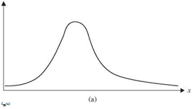
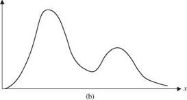
Referring to Fig. 2.12, a PDF could be unimodal with a single peak, bimodal with two peaks, or multimodal with multiple peaks. Generally, the mean, median, and mode of a random variable are different unless the PDF is symmetric and unimodal. Descriptors for the central tendency of a random variable are summarized in Table 2.1.

Example 2.10 (after Tung and Yen, 2005) Refer to Example 2.8, the pump reliability problem. Find the mean, mode, median, and 10 percent quantile for the random time to failure T.

Solution The mean of the time to failure, called the mean time to failure (MTTF), is the first-order moment about the origin, which is /xt —1250 h as calculated previ­ously in Example 2.8. From the shape of the PDF for the exponential distribution as shown in Fig. 2.7, one can immediately identify that the mode, representing the most likely time of pump failure, is at the beginning of pump operation, that is,

Подпись:

Подпись: t

mo

Подпись: fx(x)
Ш

Mean, mode, median, and quantiles

Figure 2.12 Unimodal (a) and bimodal (b) distributions.


To determine the median time to failure of the pump, one can first derive the expression for the CDF from the given exponential PDF as

rt e-u/1250

Ft(t) = P(T < t) = ————– du = 1 – e-t/1250 for t > 0

к 1250 –

in which u is a dummy variable. Then the median time to failure tmd can be obtained, according to Eq. (2.33), by solving

Ft(tmd) = 1 – exp(-tmd/1250) = 0.5 which yields tmd = 866.43 h.

Similarly, the 10 percent quantile t0.1, namely, the elapsed time over which the pump would fail with a probability of 0.1, can be found in the same way as the median except that the value of the CDF is 0.1, that is,

Ft(t0.1) = 1 – exp(-0.1/1250) = 0.1 which yields t0.1 = 131.7 h.

Statistical Properties of Random Variables

In statistics, the term population is synonymous with the sample space, which describes the complete assemblage of all the values representative of a partic­ular random process. A sample is any subset of the population. Furthermore, parameters in a statistical model are quantities that are descriptive of the pop­ulation. In this book, Greek letters are used to denote statistical parameters. Sample statistics, or simply statistics, are quantities calculated on the basis of sample observations.

2.1.3 Statistical moments of random variables

In practical statistical applications, descriptors commonly used to show the sta­tistical properties of a random variable are those indicative of (1) the central tendency, (2) the dispersion, and (3) the asymmetry of a distribution. The fre­quently used descriptors in these three categories are related to the statistical moments of a random variable. Currently, two types of statistical moments are used in hydrosystems engineering applications: product-moments and L-moments. The former is a conventional one with a long history of practice, whereas the latter has been receiving great attention recently from water re­sources engineers in analyzing hydrologic data (Stedinger et al., 1993; Rao and Hamed 2000). To be consistent with the current general practice and usage, the terms moments and statistical moments in this book refer to the conventional product-moments unless otherwise specified.

Product-moments. The r th-order product-moment of a random variable X about any reference point X = xo is defined, for the continuous case, as

/

СО /* CO

(x — xo)r fx(x) dx = / (x — xo)r dFx(x) (2.20a)

-O J — O

whereas for the discrete case,

K

E [(X — xo)r ] = ]T (xk — xo )rpx (xk) (2.20b)

k = і

where E [■] is a statistical expectation operator. In practice, the first three mo­ments (r = 1,2, 3) are used to describe the central tendency, variability, and asymmetry of the distribution of a random variable. Without losing generality, the following discussions consider continuous random variables. For discrete random variables, the integral sign is replaced by the summation sign. Here it is convenient to point out that when the PDF in Eq. (2.20a) is replaced by a conditional PDF, as described in Sec. 2.3, the moments obtained are called the conditional moments.

Since the expectation operator E [ ] is for determining the average value of the random terms in the brackets, the sample estimator for the product-moments for p’r = E(Xr), based on n available data (x1, x2,…, xn), can be written as

n

p’r = ^2 wi (n) xr (2.21)

i = 1

where wi(n) is a weighting factor for sample observation xi, which depends on sample size n. Most commonly, wi(n) = 1/n, for all i = 1, 2,…, n. The last column of Table 2.1 lists the formulas applied in practice for computing some commonly used statistical moments.

Two types of product-moments are used commonly: moments about the ori­gin, where xo = 0, and central moments, where xo = px, with px = E[X]. The r th-order central moment is denoted as pr = E [(X — px )r ], whereas the r th – order moment about the origin is denoted as p’r = E(Xr). It can be shown easily, through the binomial expansion, that the central moments pr = E [(X — px)r ] can be obtained from the moments about the origin as

r

pr = ]T( —1)fCr, i p’x ri—i (2.22)

i = 0

where Cr, i = (r) = i!(/^is a binomial coefficient, with! representing factorial, that is, r! = r x (r — 1) x (r — 2) x-x 2 x 1. Conversely, the moments about the origin can be obtained from the central moments in a similar fashion as

r

jXr = ‘У ^ Cr, i №x №r —i (2.23)

i = 0

Moment

Measure of

Definition

Continuous variable

Discrete variable

Sample estimator

First

Central

Mean, expected value

Vx = f ° xfx(x) dx

Vx = Eallx’s xkP(xk )

x = E xi/n

location

E( X) = Vx

Second

Dispersion

Variance, Var(X) = V2 = °X

ax = /Too (x – Vx)2 f x(x) dx

°x = Eallx’s(xk – Vx)2 Px(xk )

s2 = n-1 E(xi – x)2

Standard deviation, ax

ax = у/Var( X)

ax = у/Var( X)

s=J n-л E( xi – x)2

Coefficient of variation, &x

£2x = ax/vx

£2x = ax/Vx

Cv = s/x

Third

Asymmetry

Skewness

V3 = f-T (x – Vx )3 fx(x) dx

V3 = ^ ^all x’s (xk – Vx ) px(xk )

m3 = (n-1)(n-2) E (x x)

Skewness coefficient, yx

Yx = V3/a£

Yx = V3 /a£

g = m3/s’3

Fourth

Peakedness

Kurtosis, кх

V4 = 1° (x – Vx )4 fx(x) dx

V4 = allx’s (xk – V%)4px(xk )

m4 = (n-l)(n-2)(n-3) E(x x)

Excess coefficient, Ex

Kx = V4/a£

Kx = V4/a£

k = m4/s4

єx — Kx 3

Єx — Kx 3


Подпись: 37

Equation (2.22) enables one to compute central moments from moments about the origin, whereas Eq. (2.23) does the opposite. Derivations for the expressions of the first four central moments and the moments about the origin are left as exercises (Problems 2.10 and 2.11).

The main disadvantages of the product-moments are (1) that estimation from sample observations is sensitive to the presence of extraordinary values (called outliers) and (2) that the accuracy of sample product-moments deteriorates rapidly with an increase in the order of the moments. An alternative type of moments, called L-moments, can be used to circumvent these disadvantages.

Example 2.8 (after Tung and Yen, 2005) Referring to Example 2.6, determine the first two moments about the origin for the time to failure of the pump. Then calculate the first two central moments.

Solution From Example 2.6, the random variable T is the time to failure having an exponential PDF as

ft(t) = ^ exp(-1/1250) for t > 0, в> 0

in which t is the elapsed time (in hours) before the pump fails, and в = 1250 h/failure.

The moments about the origin, according to Eq. (2.20a), are

r / e-t/e

E (Tr) = t4 = J t4—J dt

Using integration by parts, the results of this integration are for r = 1, p^ = E(T ) = pt = в = 1250 h

for r = 2, p’2 = E(T 2) = 2в2 = 3,125,000 h2

Based on the moments about the origin, the central moments can be determined, according to Eq. (2.22) or Problem (2.10), as

for r = 1, P1 = E (T — pt) = 0

for r = 2, p2 = E [(T — pt )2] = p’2 — P2 = 2в2 — в2 = в2 = 1, 562, 500 h2

L-moments. The r th-order L-moments are defined as (Hosking, 1986, 1990)

Xr = 1 ^ (—1)j— ^ E (— j r) r = 1,2,… (2.24)

in which Xj :n is the j th-order statistic of a random sample of size n from the

distribution Fx(x), namely, X(1) < X(2) < ■ ■ ■ < X(j) < — < X(n). The “L” in L-moments emphasizes that Xr is a linear function of the expected order statis­tics. Therefore, sample L-moments can be made a linear combination of the ordered data values. The definition of the L-moments given in Eq. (2.24) may appear to be mathematically perplexing; the computations, however, can be sim­plified greatly through their relations with the probability-weighted moments,
which are defined as (Greenwood et al., 1979)

Подпись:xr [Fx(x)]p [1 – Fx(x)]q dFx(x)

(2.25)

Compared with Eq. (2.20a), one observes that the conventional product – moments are a special case of the probability-weighted moments with p = q = 0, that is, Mr,0,0 = g’r. The probability-weighted moments are particularly attractive when the closed-form expression for the CDF of the random variable is available.

To work with the random variable linearly, M1,p, q can be used. In particu­lar, two types of probability-weighted moments are used commonly in practice, that is,

ar = M1,0,r = E{X[1 – Fx(X)]r} r = 0,1,2,… (2.26a)

вг = M1,r,0 = E{X[Fx(X)]r} r = 0,1,2,… (2.26b)

In terms of ar or er, the r th-order L-moment Xr can be obtained as (Hosking,

1986)

Подпись: (2.27)Xr + 1 = ( -1)rJ2 Pr, j a j =Yj Pr, j ej r = 0,1 …

j = 0 j = 0

in which

Подпись: p;, j = (-1)r - jrfr + i (-1)r j (r + j )!

JA j J (j!)2(r – j)!

For example, the first four L-moments of random variable X are

X1 — e0 — g-1 — gx

(2.28a)

X2 = 2в1 – в0

(2.28b)

X3 = 6в2 – 6в1 + в0

(2.28c)

X4 = 20вэ – 30в2 + 12в1 – в0

(2.28d)

To estimate sample a – and в-moments, random samples are arranged in as­cending or descending order. For example, arranging n random observations in ascending order, that is, X(1) < X(2) < ■ ■ ■ < X(j) < ■ ■ ■ < X(n), the rth-order в-moment er can be estimated as

1n

er = -]T X(i) F (X(i))r (2.29)

n

i = 1

where F(X(i)) is an estimator for F(X(i>) = P(X < X(i>), for which many plotting-position formulas have been used in practice (Stedinger et al., 1993).

The one that is used often is the Weibull plotting-position formula, that is,

F (X (i)) = i / (n + 1).

L-moments possess several advantages over conventional product-moments. Estimators of L-moments are more robust against outliers and are less biased. They approximate asymptotic normal distributions more rapidly and closely. Although they have not been used widely in reliability applications as com­pared with the conventional product-moments, L-moments could have a great potential to improve reliability estimation. However, before more evidence be­comes available, this book will limit its discussions to the uses of conventional product-moments.

Example 2.9 (after Tung and Yen, 2005) Referring to Example 2.8, determine the first two L-moments, that is, Л1 and Л2, of random time to failure T.

Solution To determine Л1 and Л2, one first calculates 0o and 01, according to Eq. (2.26b), as

0 = E{T [Ft(T)]0} = E(T) = nt = в

Подпись: рЖ рЖ E {T [Ft (T )^}= / [t Ft (t)] ft (t) dt = [t(1 - e-t/0 )](e—t/0/0) dt = 40 00 01 =

00 From Eq. (2.28), the first two L-moments can be computed as

Подпись: ^1 = 0O = nt = 160 0

Л2 = 201 – 00 = —— 0 = —

Joint, conditional, and marginal distributions

The joint distribution and conditional distribution, analogous to the concepts of joint probability and conditional probability, are used for problems involving multiple random variables. For example, flood peak and flood volume often are considered simultaneously in the design and operation of a flood-control reservoir. In such cases, one would need to develop a joint PDF of flood peak and flood volume. For illustration purposes, the discussions are limited to problems involving two random variables.

The joint PMF and joint CDF of two discrete random variables X and Y are defined, respectively, as

px, y(x, y) = P(X = x, Y = y) (2.14a)

Fx, y(u, v) = P(X < u, Y < v) = px, y(x, y) (2.14b)

x<u y<v

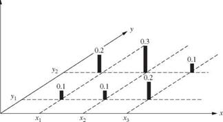
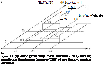
Schematic diagrams of the joint PMF and joint CDF of two discrete random variables are shown in Fig. 2.8.

Px, y(x, y)

Joint, conditional, and marginal distributions

(a)


Fx, y(x, y)

Joint, conditional, and marginal distributions Подпись: (2.15a) (2.15b)

The joint PDF of two continuous random variables X and Y, denoted as fx, y( x, y), is related to its corresponding joint CDF as

Similar to the univariate case, Fx, y(—TO, —to) = 0 and Fx, у(то, to) = 1. Two ran­dom variables X and Y are statistically independent if and only if fx, y(x, y) = fx(x) x fy(y) and Fx, y(x, y) = Fx(x) x Fy(y). Hence a problem involving multi­ple independent random variables is, in effect, a univariate problem in which each individual random variable can be treated separately.

Подпись: fx ( x) Подпись: fx, y( x, y) dy Подпись: (2.16)

If one is interested in the distribution of one random variable regardless of all others, the marginal distribution can be used. Given the joint PDF fx, y(x, y), the marginal PDF of a random variable X can be obtained as

For continuous random variables, the conditional PDF for X | Y, similar to the conditional probability shown in Eq. (2.6), can be defined as

fx (x | y) = ff (*f (2.17)

fy(y)

in which fy( y) is the marginal PDF of random variable Y. The conditional PMF for two discrete random variables similarly can be defined as

, , ч px, y(x y) ,Q1{n

px(x | y) = —, (2.18)

py(y)

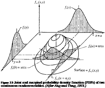
Figure 2.9 shows the joint and marginal PDFs of two continuous random vari­ables X and Y. It can be shown easily that when the two random variables are statistically independent, fx(x | y) = fx(x).

Equation (2.17) alternatively can be written as

fx, y(x, y) = fx(x | y) X fy(y) (2.19)

Подпись:
which indicates that a joint PDF between two correlated random variables can be formulated by multiplying a conditional PDF and a suitable marginal PDF.

Note that the marginal distributions can be obtained from the joint distribution function, but not vice versa.

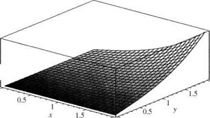
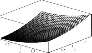
Example 2.7 Suppose that X and Y are two random variables that can only take values in the intervals 0 < x < 2 and 0 < y < 2. Suppose that the joint CDF of X and Y for these intervals has the form of Fx, y(x, y) = cxy(x2 + y2). Find (a) the joint PDF of X and Y, (b) the marginal PDF of X, (c) the conditional PDF fy(y | x = 1), and (d) P(Y < 11 x = 1).

Solution First, one has to find the constant c so that the function Fx, y(x, y) is a legit­imate CDF. It requires that the value of Fx, y(x, y) = 1 when both arguments are at their respective upper bounds. That is,

Fxy(x = 2, y = 2) = 1 = c(2)(2)(22 + 22)

Therefore, c = 1/32. The resulting joint CDF is shown in Fig. 2.10a.

Joint, conditional, and marginal distributions

Fx, y (x, y) 1

0.8

0.6

0.4

0.2


2


2 0 (a)


fx, y (x, y)

0.7 0.6 0.5 – 0.4 – 0.3 0.2 ■ 0.1 0

0


2


2 0 (b)


Figure 2.10 (a) Joint cumulative distribution function (CDF) and (b) probability density function (PDF) for Example 2.7.


Joint, conditional, and marginal distributionsJoint, conditional, and marginal distributions

(a)

Joint, conditional, and marginal distributions Joint, conditional, and marginal distributions Joint, conditional, and marginal distributions Подпись: for 0 < x, y < 2

To derive the joint PDF, Eq. (2.15a) is applied, that is,

A plot of joint PDF is shown in Fig. 2.10b.

(b) To find the marginal distribution of X, Eq. (2.16) can be used:

f2 3(x2 + y2) 4 + 3×2

Подпись: 32Подпись: 16fx(x) = —– —— dx = ——— for 0 < x < 2

0

fy( y 1 x = 1) =

(c)

Joint, conditional, and marginal distributions Подпись: for 0 < y < 2

The conditional distribution fy(y | x) can be obtained by following Eq. (2.17) as

(d) The conditional probability P(Y < 11 X = 1) can be computed as

P(Y < 11 X = 1) = £ fy(y | x = 1) dy = £ 3(1+4y2} dy = 7