Binomial distribution
The binomial distribution is applicable to random processes with only two types of outcomes. The state of components or subsystems in many hydrosystems can be classified as either functioning or failed, which is a typical example of a binary outcome. Consider an experiment involving a total of n independent trials with each trial having two possible outcomes, say, success or failure. In each trial, if the probability of having a successful outcome is p, the probability of having x successes in n trials can be computed as
Px(x) = Cn, xpxqn-x for x = 0,1,2,…,n (2.51)
where Cn, x is the binomial coefficient, and q = 1 – p, the probability of having a failure in each trial. Computationally, it is convenient to use the following recursive formula for evaluating the binomial PMF (Drane et al., 1993):
Px(x | n, p) = (——————- x——– JVqjPx(x — 11 n, p) = Rb(x)Px(x — 11 n, p) (2.52)
for x = 0, 1,2,…, n, with the initial probability px(x = 0|n, p) = qn. A simple recursive scheme for computing the binomial cumulative probability is given by Tietjen (1994).
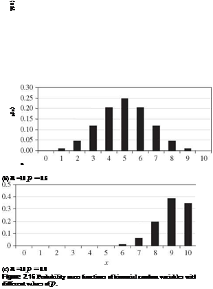
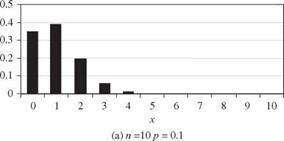
A random variable X having a binomial distribution with parameters n and p has the expectation E (X) = np and variance Var(X) = npq. Shape of the PMF of a binomial random variable depends on the values of p and q. The skewness coefficient of a binomial random variable is (q — p)/^/npq. Hence the PMF is positively skewed if p <q, symmetric if p = q = 0.5, and negatively skewed if p > q. Plots of binomial PMFs for different values of p with a fixed n are shown in Fig. 2.16. Referring to Fig. 2.15, the sum of several independent binomial random variables, each with a common parameter p and different nk s, is still a binomial random variable with parameters p and £knk.
Example 2.14 A roadway-crossing structure, such as a bridge or a box or pipe culvert, is designed to pass a flood with a return period of 50 years. In other words, the annual probability that the roadway-crossing structure would be overtopped is a 1-in-50 chance or 1/50 = 0.02. What is the probability that the structure would be overtopped over an expected service life of 100 years?
Solution In this example, the random variable X is the number of times the roadwaycrossing structure will be overtopped over a 100-year period. One can treat each year as an independent trial from which the roadway structure could be overtopped or not overtopped. Since the outcome of each “trial” is binary, the binomial distribution is applicable.

 |

The event of interest is the overtopping of the roadway structure. The probability of such an event occurring in each trial (namely, each year), is 0.02. A period of 100 years represents 100 trials. Hence, in the binomial distribution model, the parameters are p = 0.02 and n = 100. The probability that overtopping occurs in a period of 100 years can be calculated, according to Eq. (2.51), as
P (overtopping occurs in an 100-year period)
= P (overtopping occurs at least once in an 100-year period)
= P(X > 11 n = 100, p = 0.02)
100 100
= X) Px(x) = X) C1°°>x(0.02)x(0.98)100-x
x = 1 x = 1
This equation for computing the overtopping probability requires evaluations of 100 binomial terms, which could be very cumbersome. In this case, one could solve the problem by looking at the other side of the coin, i. e., the nonoccurrence of overtopping events. In other words,
P (overtopping occurs in a 100-year period)
= P (overtopping occurs at least once in a 100-year period)
= 1 — P (no overtopping occurs in a 100-year period)
= 1 — p( X = 0) = 1 — (0.98)100
= 1 — 0.1326 = 0.8674
Calculation of the overtopping risk, as illustrated in this example, is made under an implicit assumption that the occurrence of floods is a stationary process. In other words, the flood-producing random mechanism for the watershed under consideration does not change with time. For a watershed undergoing changes in hydrologic characteristics, one should be cautious about the estimated risk.
The preceding example illustrates the basic application of the binomial distribution to reliability analysis. A commonly used alternative is the Poisson distribution described in the next section. More detailed descriptions of these two distributions in time-dependent reliability analysis of hydrosystems infrastructural engineering are given in Sec. 4.7.


Leave a reply