Joint, conditional, and marginal distributions
The joint distribution and conditional distribution, analogous to the concepts of joint probability and conditional probability, are used for problems involving multiple random variables. For example, flood peak and flood volume often are considered simultaneously in the design and operation of a flood-control reservoir. In such cases, one would need to develop a joint PDF of flood peak and flood volume. For illustration purposes, the discussions are limited to problems involving two random variables.
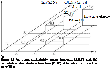
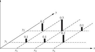
The joint PMF and joint CDF of two discrete random variables X and Y are defined, respectively, as
px, y(x, y) = P(X = x, Y = y) (2.14a)
Fx, y(u, v) = P(X < u, Y < v) = px, y(x, y) (2.14b)
x<u y<v
Schematic diagrams of the joint PMF and joint CDF of two discrete random variables are shown in Fig. 2.8.
Px, y(x, y)
|
Fx, y(x, y)
 |
|
The joint PDF of two continuous random variables X and Y, denoted as fx, y( x, y), is related to its corresponding joint CDF as
Similar to the univariate case, Fx, y(—TO, —to) = 0 and Fx, у(то, to) = 1. Two random variables X and Y are statistically independent if and only if fx, y(x, y) = fx(x) x fy(y) and Fx, y(x, y) = Fx(x) x Fy(y). Hence a problem involving multiple independent random variables is, in effect, a univariate problem in which each individual random variable can be treated separately.
If one is interested in the distribution of one random variable regardless of all others, the marginal distribution can be used. Given the joint PDF fx, y(x, y), the marginal PDF of a random variable X can be obtained as
For continuous random variables, the conditional PDF for X | Y, similar to the conditional probability shown in Eq. (2.6), can be defined as
fx (x | y) = ff (*f (2.17)
fy(y)
in which fy( y) is the marginal PDF of random variable Y. The conditional PMF for two discrete random variables similarly can be defined as
, , ч px, y(x y) ,Q1{n
px(x | y) = —, (2.18)
py(y)
Figure 2.9 shows the joint and marginal PDFs of two continuous random variables X and Y. It can be shown easily that when the two random variables are statistically independent, fx(x | y) = fx(x).
Equation (2.17) alternatively can be written as
fx, y(x, y) = fx(x | y) X fy(y) (2.19)
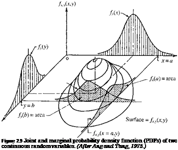
which indicates that a joint PDF between two correlated random variables can be formulated by multiplying a conditional PDF and a suitable marginal PDF.
Note that the marginal distributions can be obtained from the joint distribution function, but not vice versa.
Example 2.7 Suppose that X and Y are two random variables that can only take values in the intervals 0 < x < 2 and 0 < y < 2. Suppose that the joint CDF of X and Y for these intervals has the form of Fx, y(x, y) = cxy(x2 + y2). Find (a) the joint PDF of X and Y, (b) the marginal PDF of X, (c) the conditional PDF fy(y | x = 1), and (d) P(Y < 11 x = 1).
Solution First, one has to find the constant c so that the function Fx, y(x, y) is a legitimate CDF. It requires that the value of Fx, y(x, y) = 1 when both arguments are at their respective upper bounds. That is,
Fxy(x = 2, y = 2) = 1 = c(2)(2)(22 + 22)
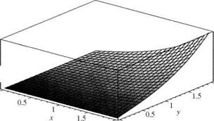
Therefore, c = 1/32. The resulting joint CDF is shown in Fig. 2.10a.

|
|
|
|
|
|
|
|
|
|
|
|
|
(a)
To derive the joint PDF, Eq. (2.15a) is applied, that is,
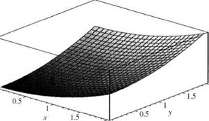
A plot of joint PDF is shown in Fig. 2.10b.
(b) To find the marginal distribution of X, Eq. (2.16) can be used:
f2 3(x2 + y2) 4 + 3×2
![]()
![]() fx(x) = —– —— dx = ——— for 0 < x < 2
fx(x) = —– —— dx = ——— for 0 < x < 2
0
|
fy( y 1 x = 1) = |
(c)
The conditional distribution fy(y | x) can be obtained by following Eq. (2.17) as
(d) The conditional probability P(Y < 11 X = 1) can be computed as
P(Y < 11 X = 1) = £ fy(y | x = 1) dy = £ 3(1+4y2} dy = 7


Leave a reply