Category Hydrosystems Engineering Reliability Assessment and Risk Analysis

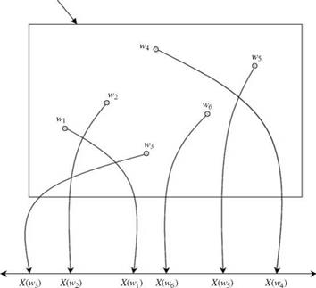
In analyzing the statistical features of infrastructural system responses, many events of interest can be defined by the related random variables. A random variable is a real-value function defined on the sample space. In other words, a random variable can be viewed as a mapping from the sample space to the real line, as shown in Fig. 2.4. The standard convention is to denote a random variable by an upper-case letter, whereas a lower-case letter is used to repre­sent the realization of the corresponding random variable. For example, one may use Q to represent flow magnitude, a random variable, whereas q is used to represent the values that Q takes. A random variable can be discrete or con­tinuous. Examples of discrete random variables encountered in hydrosystems infrastructural designs are the number of storm events occurring in a specified time period, the number of overtopping events per year for a levee system, and so on. On the other hand, examples of continuous random variables are flow rate, rainfall intensity, water-surface elevation, roughness factor, and pollution concentration, among others.

2.1.2 Cumulative distribution function

and probability density function

The cumulative distribution function (CDF), or simply distribution function (DF), of a random variable X is defined as

Fx (x) = P (X < x)

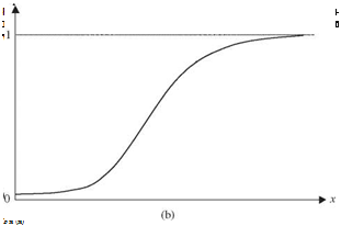
The CDF Fx(x) is the nonexceedance probability, which is a nondecreasing function of the argument x, that is, Fx(a) < Fx(b), for a < b. As the argument x approaches the lower bounds of the random variable X, the value of Fx (x) approaches zero, that is, limx^-x Fx(x) = 0; on the other hand, the value of Fx(x) approaches unity as its argument approaches the upper bound of X, that is, limx^cx, Fx (x) = 1. With a < b, P (a < X < b) = Fx (b) – Fx (a).

For a discrete random variable X, the probability mass function (PMF), is defined as

Px (x) = P (X = x) (2.11)

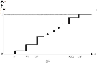
The PMF of any discrete random variable, according to axioms (1) and (2) in Sec. 2.1, must satisfy two conditions: (1) px(xk) > 0, for all xk’s, and (2) Sail kpx(xk) = 1. The PMF of a discrete random variable and its associated CDF are sketched schematically in Fig. 2.5. As can be seen, the CDF of a dis­crete random variable is a staircase function.

For a continuous random variable, the probability density function (PDF) fx( x) is defined as

The PDF of a continuous random variable f x (x) is the slope of its corresponding CDF. Graphic representations of a PDF and a CDF are shown in Fig. 2.6. Similar to the discrete case, any PDF of a continuous random variable must satisfy two conditions: (1) fx(x) > 0 and (2) / fx(x) dx = 1. Given the PDF of a random variable X, its CDF can be obtained as

x

fx(u) du

-TO

in which u is the dummy variable. It should be noted that fx ( ) is not a prob­ability; it only has meaning when it is integrated between two points. The probability of a continuous random variable taking on a particular value is zero, whereas this may not be the case for discrete random variables.

Example 2.6 The time to failure T of a pump in a water distribution system is a continuous random variable having the PDF of

ft(t) = exp(-t/1250)/e for t > 0, в > 0

in which t is the elapsed time (in hours) before the pump fails, and в is the parameter of the distribution function. Determine the constant в and the probability that the operating life of the pump is longer than 200 h.

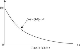
Solution The shape of the PDF is shown in Fig. 2.7. If the function ft (t) is to serve as a PDF, it has to satisfy two conditions: (1) ft(t) > 0, for all t, and (2) the area under ft (t) must equal unity. The compliance of the condition (1) can be proved easily. The value of the constant в can be determined through condition (2) as

1=
в
0

Therefore, the constant в = 1250 h/failure. This particular PDF is called the exponen­tial distribution (see Sec. 2.6.3). To determine the probability that the operational life of the pump would exceed 200 h, one calculates P (T > 200):

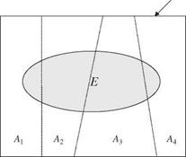
The probability of the occurrence of an event E, in general, cannot be deter­mined directly or easily. However, the event E may occur along with other attribute events Ak. Referring to Fig. 2.2, event E could occur jointly with K mutually exclusive (Aj П Ak — 0 for j — k) and collectively exhaustive (A1 U A2 U—U AK) — S attributes Ak, k — 1,2,…, K. Then the probability of the occur­rence of an event E, regardless of the attributes, can be computed as

KK

P(E) — P(E, Ak) — P (E | Ak)P(Ak) (2.8)

k—1 k—1

Equation (2.8) is called the total probability theorem.

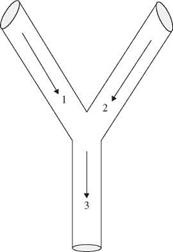
Example 2.4 Referring to Fig. 2.3, two upstream storm sewer branches (I1 and I2) merge to a sewer main (I3). Assume that the flow-carrying capacities of the two up­stream sewer branches I1 and I2 are equal. However, hydrologic characteristics of the contributing drainage basins corresponding to I1 and I2 are somewhat differ­ent. Therefore, during a major storm event, the probabilities that sewers I1 and I2 will exceed their capacities (surcharge) are 0.5 and 0.4, respectively. For simplicity, assume that the occurrences of surcharge events in the two upstream sewer branches are independent of each other. If the flow capacity of the downstream sewer main I3 is

Figure 2.3 A system with three sewer sections.

the same as its two upstream branches, what is the probability that the flow capacity of the sewer main I3 will be exceeded? Assume that when both upstream sewers are carrying less than their full capacities, the probability of downstream sewer main I3 exceeding its capacity is 0.2.

Solution Let E1, E2, and E3, respectively, be events that sewer I1, I2, and I3 exceed their respective flow capacity. From the problem statements, the following probabili­ties can be identified: P(E1) = 0.50, P(E2) = 0.40, and P(E3 | E1, E’2) = 0.2.

To determine P(E3), one first considers the basic events occurring in the two up­stream sewer branches that would result in surcharge in the downstream sewer main E3. There are four possible attribute events that can be defined from the flow con­ditions of the two upstream sewers leading to surcharge in the downstream sewer main. They are A1 = (E1, E2), A2 = (E1, E2), A3 = (E1, E2), and A4 = (E1, E2). Fur­thermore, the four events A1, A2, A3, and A4 are mutually exclusive.

Since the four attribute events A1, A2, A3, and A4 contribute to the occurrence of event E3, the probability of the occurrence of E3 can be calculated, according to Eq. (2.8), as

P(E3) = P(E3, A1) + P(E3, A2) + P(E3, A3) + P(E3, A4)

= P(E3 | A1)P(A1) + P(E3 | A2)P(A2) + P(E3 | A3)P(A3) + P(E3 | A4)P(A4)

To solve this equation, each of the probability terms on the right-hand side must be identified. First, the probability of the occurrence of A1, A2, A3, and A4 can be determined as the following:

P(A1) = P(E1, E2) = P(E1) x P(E2) = (0.5)(0.4) = 0.2

The reason that P (E1, E2) = P (E1) x P (E2) is due to the independence of events E1 and E2. Since E1 and E2 are independent events, then E1, E1, E2, and E2 are also

independent events. Therefore,

P(A2) = P(E, E2) = P() x P(E2) = (1 – 0.5)(0.4) = 0.2

P(A3) = P(E1, E2) = P(E1) x P(E2) = (0.5)(1 – 0.4) = 0.3

P(A4) = P(E1, E2) = P(E1) x P(E2) = (1 – 0.5)(1 – 0.4) = 0.3

The next step is to determine the values of the conditional probabilities, that is, P(E3 | A1), P(E3 | A2), P(E3 | A3), and P(E3 | A4). The value of P(E3 | A4) = P(E3 | E’, E2) = 0.2 is given by the problem statement. On the other hand, the values of the remaining three conditional probabilities can be determined from an understanding of the physical process. Note that from the problem statement the downstream sewer main has the same conveyance capacity as the two upstream sewers. Hence any up­stream sewer exceeding its flow-carrying capacity would result in surcharge in the downstream sewer main. Thus the remaining three conditional probabilities can be easily determined as

P(E3 | A1) = P(E3 | E1, E2) = 1.0 P(E3 | A2) = P(E3 | E1, E2) = 1.0 P(E3 | A3) = P(E3 | E1, E2) = 1.0

Putting all relevant information into the total probability formula given earlier, the probability that the downstream sewer main I3 would be surcharged in a major storm is

P(E3) = P(E3 | A1)P(A1) + P(E3 | A2)P(A2) + P(E3 | A3)P(A3) + P(E3 | A4)P(A4)

= (1.0)(0.2) + (1.0)(0.2) + (1.0)(0.3) + (0.2)(0.3)

= 0.76

The total probability theorem describes the occurrence of an event E that may be affected by a number of attribute events Ak, k = 1, 2,…, K. In some situations, one knows P (E | Ak) and would like to determine the probability that a particular event Ak contributes to the occurrence of event E. In other words, one likes to find P(Ak | E). Based on the definition of the conditional probability (Eq. 2.6) and the total probability theorem (Eq. 2.8), P (Ak | E) can be computed as

Equation (2.9) is called Bayes’ theorem, and P (Ak) is the prior probability, rep­resenting the initial belief of the likelihood of occurrence of attribute event Ak. P (E | Ak) is the likelihood function, and P (Ak | E) is the posterior probability, representing the new evaluation of Ak being responsible in the light of the oc­currence of event E. Hence Bayes’ theorem can be used to update and revise the calculated probability as more information becomes available.

Example 2.5 Referring to Example 2.4, if surcharge is observed in the downstream storm sewer main I3, what is the probability that the incident is caused by simulta­neous surcharge of both upstream sewer branches?

Solution From Example 2.4, A1 represents the event that both upstream storm sewer branches exceed their flow-carrying capacities. The problem is to find the conditional probability of A1, given that event E3 has occurred, that is, P(A1 | E3). This condi­tional probability can be expressed as

From Example 2.4, the numerator and denominator of the preceding conditional prob­ability can be computed as

The original assessment of the probability is 20 percent that both upstream sewer branches would exceed their flow-carrying capacities. After an observation of down­stream surcharge from a new storm event, the probability of surcharge occurring in both upstream sewers is revised to 26.3 percent.

The conditional probability is the probability that a conditional event would occur. The conditional probability P (A | B) can be computed as

P(AI B) = PAA <2.6)

in which P (A | B) is the occurrence probability of event A given that event B has occurred. It represents a reevaluation of the occurrence probability of event A in the light of the information that event B has occurred. Intuitively, A and B are two independent events if and only if P (A | B) = P (A). In many cases it is convenient to compute the joint probability P (A, B) by

P (A, B) = P (B) P (A | B) or P (A, B) = P (A) P (B | A)

The probability of the joint occurrence of K dependent events can be general­ized as

Example 2.3 Referring to Example 2.2, the probabilities that tributaries i and 2 would overflow during a major storm event are 0.5 and 0.4, respectively. After exam­ining closely the assumption about the independence of overflow events in the two tributaries, its validity is questionable. Through an analysis of historical overflow events, it is found that the probability of tributary 2 overflowing is 0.6 if tributary i overflows. Determine the probability that at least one tributary would overflow in a major storm event.

Solution Let Ei and E2 be the events that tributary i and 2 overflow, respectively. From the problem statement, the following probabilities can be identified:

P(Ei) = 0.5 P(E2) = 0.4 P(E2 | Ei) = 0.6

in which P(E2 | Ei) is the conditional probability representing the likelihood that tributary 2 would overflow given that tributary i has overflowed. The probability of at least one tributary overflowing during a major storm event can be computed by

P(Ei U E2) = P(Ei) + P(E2) – P(Ei, E2)

in which the probability of joint occurrence of both tributaries overflowing, that is, P(E1, E2), can be obtained from the given conditional probability, according to Eq. (2.7), as

P(E1, E2) — P(E2 | E1)P(E1) — (0.6)(0.5) — 0.3

The probability that at least one tributary would overflow during a major storm event can be obtained as

P(E1 U E2) — P(E1) + P(E2) – P(E1, E2) — 0.5 + 0.4 – 0.3 — 0.6

If two events are statistically independent of each other, the occurrence of one event has no influence on the occurrence of the other. Therefore, events A and B are independent if and only if P (A, B) = P (A) P (B). The probability of joint occurrence of K independent events can be generalized as

K

= P(A1) X P(A2) x-.-x P(Ak) = П P(Ak)

k=1

It should be noted that the mutual exclusiveness of two events does not, in general, imply independence, and vice versa, unless one of the events is an impossible event. If the two events A and B are independent, then A, A7, B, and B’ all are independent, but not necessarily mutually exclusive, events.

Example 2.2 Referring to Example 2.1, the probabilities that tributaries 1 and 2 overflow during a major storm event are 0.5 and 0.4, respectively. For simplicity, assume that the occurrences of overflowing in the two tributaries are independent of each other. Determine the probability of at least one tributary overflowing in a major storm event.

Solution Use the same definitions for events E1 and E2. The problem is to determine P(E1 U E2) by

P(E1 U E2) = P(E1) + P(E2) – P(E1, E2)

Note that in this example the probability of joint occurrences of both tributaries over­flowing, that is, P(E1, E2), is not given directly by the problem statement, as in Example 2.1. However, it can be determined from knowing that the occurrences of
overflows in the tributaries are independent events, according to Eq. (2.5), as

P(Ex, E2) = P(E1)P(E2) = (0.5)(0.4) = 0.2

Then the probability that at least one tributary would overflow during a major storm event is

P(Ei U E2) = P(Ei) + P(E2) – P(Ex, E2) = 0.5 + 0.4 – 0.2 = 0.7

2.1.1 Basic axioms of probability

The three basic axioms of probability computation are (1) nonnegativity: P (A) > 0, (2) totality: P (S) = 1, with S being the sample space, and (3) additivity: For two mutually exclusive events A and B, P(A U B) = P(A) + P(B).

As indicated from axioms (1) and (2), the value of probability of an event occurring must lie between 0 and 1. Axiom (3) can be generalized to consider K mutually exclusive events as

P (A1 U A2 U-.-U Ak ) = p( U aA =£) P (Ak) (2.2)

‘vk=1 ‘ k=1

An impossible event is an empty set, and the corresponding probability is zero, that is, P(0) = 0. Therefore, two mutually exclusive events A and B have zero probability of joint occurrence, that is, P (A, B) = P (0) = 0. Although the prob­ability of an impossible event is zero, the reverse may not necessarily be true. For example, the probability of observing a flow rate of exactly 2000 m3/s is zero, yet having a discharge of 2000 m3/s is not an impossible event.

Relaxing the requirement of mutual exclusiveness in axiom (3), the probabil­ity of the union of two events can be evaluated as

P(A U B) = P(A) + P(B) – P(A, B) (2.3)

which can be further generalized as

/ K N K

W ^AkJ = £ P (Ak) – ££P ( a Aj •

^ ‘ k = 1 i < j

+ EEE P(At, A, Ak) -■ ■ ■ + (-1)KP(A1, A2,…, Ak)

i < j < k

(2.4)

If all are mutually exclusive, all but the first summation term on the right-hand side of Eq. (2.3) vanish, and it reduces to Eq. (2.2).

Example 2.1 There are two tributaries in a watershed. From past experience, the probability that water in tributary 1 will overflow during a major storm event is 0.5, whereas the probability that tributary 2 will overflow is 0.4. Furthermore, the probability that both tributaries will overflow is 0.3. What is the probability that at least one tributary will overflow during a major storm event?

Solution Define Ei = event that tributary i overflows for i = 1, 2. From the prob­lem statements, the following probabilities are known: P(E]_) = 0.5, P(E2) = 0.4, and P(E1, E2) = 0.3.

The probability having at least one tributary overflowing is the probability of event E1 or E2 occurring, that is, P(E1 U E2). Since the overflow of one tributary does not preclude the overflow of the other tributary, E1 and E2 are not mutually exclusive. Therefore, the probability that at least one tributary will overflow during a major storm event can be computed, according to Eq. (2.3), as

P(E1 U E2) = P(E1) + P(E2) – P(E1, E2) = 0.5 + 0.4 – 0.3 = 0.6

Assessment of the reliability of a hydrosystems infrastructural system or its components involves the use of probability and statistics. This chapter reviews and summarizes some fundamental principles and theories essential to relia­bility analysis.

2.1 Terminology

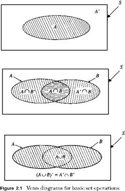
In probability theory, an experiment represents the process of making obser­vations of random phenomena. The outcome of an observation from a random phenomenon cannot be predicted with absolute accuracy. The entirety of all possible outcomes of an experiment constitutes the sample space. An event is any subset of outcomes contained in the sample space, and hence an event could be an empty (or null) set, a subset of the sample space, or the sample space itself. Appropriate operators for events are union, intersection, and com­plement. The occurrence of events A and B is denoted as A U B (the union of A and B), whereas the joint occurrence of events A and B is denoted as A n B or simply (A, B) (the intersection of A and B). Throughout the book, the comple­ment of event A is denoted as A. When two events A and B contain no common elements, then the two events are mutually exclusive or disjoint events, which is expressed as (A, B) = 0, where 0 denotes the null set. Venn diagrams illustrat­ing the union and intersection of two events are shown in Fig. 2.1. When the oc­currence of event A depends on that of event B, then they are conditional events,

*Most of this chapter, except Secs. 2.5 and 2.7, is adopted from Tung and Yen (2005).

Copyright © 2006 by The McGraw-Hill Companies, Inc. Click here for terms of use.

which is denoted by A | B. Some useful set operation rules are

1. Commutative rule: AU B = B U A; AП B = B П A.

2. Associative rule: (AU B) U C = AU (B U C); (AП B) n C = An (B n C).

3. Distributive rule: An (B U C) = (An B) U (An C); AU (B n C) = (AU B) n (A U C).

4. de Morgan’s rule: (AU BУ = An B’; (AnBУ = A’UB’.

Probability is a numeric measure of the likelihood of the occurrence of an event. Therefore, probability is a real-valued number that can be manipulated by ordinary algebraic operators, such as +, -, x, and /. The probability of the occurrence of an event A can be assessed in two ways. In the case where an experiment can be repeated, the probability of having event A occurring can be estimated as the ratio of the number of replications in which event A occurs nA versus the total number of replications n, that is, nA/n. This ratio is called the relative frequency of occurrence of event A in the sequence of n replications. In principle, as the number of replications gets larger, the value of the relative frequency becomes more stable, and the true probability of event A occurring could be obtained as

P (A) = lim„^TO—A (2.1)

n

The probabilities so obtained are called objective or posterior probabilities be­cause they depend completely on observations of the occurrence of the event.

In some situations, the physical performance of an experiment is prohibited or impractical. The probability of the occurrence of an event can only be estimated subjectively on the basis of experience and judgment. Such probabilities are called subjective or prior probabilities.

There are two basic probabilistic approaches to evaluate the reliability of an in­frastructural system. The most direct approach is a statistical analysis of data of past failure records for similar systems. The other approach is through relia­bility analysis, which considers and combines the contribution of each factor po­tentially influencing failure. The former is a lumped-system approach requiring
no knowledge about the internal physical behavior of the facility or structure and its load and resistance. For example, dam failure data show that the overall average failure probability for dams of all types over 15 m in height is around 10-3 per dam per year (U. S. National Research Council, 1983; Cheng, 1993). This statistical approach may fit well with manufactured systems for which planned repeated tests can be made and the performance of many identical prototypes can be observed. For infrastructural systems in most cases, this di­rect approach is impractical because (1) infrastructures are usually unique and site-specific, (2) the sample size is too small to be statistically reliable, especially for low-probability/high-consequence events, (3) the sample may not be repre­sentative of the structure or of the population, and (4) the physical conditions of a dam may be nonstationary, i. e., varying with respect to time. The average risk of dam failure mentioned earlier does not differentiate concrete dams from earth-fill dams, arch dams from gravity dams, large dams from small dams, and old dams from new dams. If one wished to know the likelihood of failure of a particular 10-year-old double-curvature-arch concrete high dam, most likely one will find only very few failure data of similar dams, insufficient for any meaningful statistical analysis. Since no dams are identical and conditions of dams change with time, in many circumstances it may be more desirable to use the second approach by conducting a reliability analysis.

There are two major steps in reliability analysis: (1) to identify and an­alyze the uncertainties of each contributing factor and (2) to combine the uncertainties of the stochastic factors to determine the overall reliability of the structure. The second step, in turn, also may proceed in two different ways: (1) directly combining the uncertainties of all factors and (2) separately combin­ing the uncertainties of the factors belonging to different components or subsys­tems to evaluate first the respective subsystem reliability and then combining the reliabilities of the different components or subsystems to yield the over­all reliability of the structure. The first way applies to very simple structures, whereas the second way is more suitable to complicated systems. For exam­ple, to evaluate the reliability of a dam, the hydrologic, hydraulic, geotechnical, structural, and other disciplinary reliabilities could be evaluated separately first and then combined to yield the overall dam reliability. Or the component reliabilities could be evaluated first according to the different failure modes and then combined. Analysis tools

In engineering design and analysis, loads usually arise from natural events, such as floods, storms, or earthquakes, that occur randomly in time and in space. The conventional practice for measuring the reliability of a hydrosystems engineering infrastructure is the return period or recurrence interval. The return period is defined as the long-term average (or expected) time between two successive failure-causing events. In time-to-failure analysis (Chap. 5), an equivalent term is the mean time to failure. Simplistically, the return period is equal to the reciprocal of the probability of the occurrence of the event in any one time interval. For many hydrosystems engineering applications, the time interval chosen is 1 year so that the probability associated with the return period is the average annual failure probability. Frequency analysis using the annual maximum flood or rainfall series is a typical example of this kind. Hence the determination of return period depends on the time period chosen (Borgman, 1963). The main theoretical disadvantage of using return period is that reliability is measured only in terms of expected time of occurrence of loads without considering their interactions with the resistance (Melchers, 1999).

In fact, the conventional interpretation of return period can be general­ized as the average time period or mean time of the system failure when all uncertainties affecting load and resistance are considered. In other words, the return period can be calculated as the reciprocal of the failure probabil­ity computed by Eq. (1.2). Based on this generalized notion of return period, the equivalent return period corresponding to the conventional return period under different levels of resistance uncertainty is shown in Fig. 1.7. As can be seen, the equivalent return period becomes shorter than the conventional return period, as anticipated, when resistance uncertainty increases. For exam­ple, with COV(R) = 5 percent, a hydrosystem designed with a 100-year return

TABLE 1.1 Different Types of Safety Factors

Type of safety

factor Definition

Assigned number

rr /rl, where rr and rl are the true mean values of resistance and load R/L, where R and L are the mean values of resistance and load estimated from the available data

Ro/Lo, where Ro and Lo are the specified resistance and load 1/Y = Nl/Nr, where pf = P(L > yR) = P(NlL > NrR)

SOURCE: After Yen, 1979.

period under the conventional approach actually has about a 50-year return period.

Two other types of reliability measures that consider the relative magnitudes of resistance and anticipated load (called design load) are used frequently in engineering practice. One is the safety margin (SM), defined as the difference between the resistance and the anticipated load, that is,

SM = R – L (1.4)

The other is called the safety factor (SF), a ratio of resistance to load defined as

SF = R/L (1.5)

Several types of safety factors are summarized in Table 1.1, and their applica­tions to engineering systems are discussed by Yen (1979).

Preassigned safety factor. This is an arbitrarily chosen safety factor that is used conventionally without probabilistic consideration. The value chosen largely depends on the designer’s subjective judgment with regard to the amount of uncertainty involved in his or her determination of design load and the level of safety desired.

Central safety factor. Owing to the fact that both resistance and load could be subject to uncertainty, the safety factor defined by Eq. (1.5), in fact, is a quantity subject to uncertainty as well. The central safety factor rsf is defined as

RSF = R R /RL (1.6)

in which rr and rl are the true mean values of resistance and load, respectively. In practice, values of rr and rl cannot be obtained precisely from the limited data. Therefore, rsf is only of theoretical interest.

Mean safety factor. If the estimated means of R and L on the basis of data are R and L, respectively, the mean safety factor (SF) is defined as

SF = R/L

Characteristic safety factor. Often in a project the significant design values of the parameters are not the mean values but specified values (or range of values). For example, the load used in a spillway design is not the mean value of all the floods nor the mean value of the selected floods of an annual maximum series. It may be simply a specified flood of a given magnitude (e. g., a flood with a 100-year return period). Therefore, the characteristic safety factor (SFc) can be defined as

SFc = Ro/Lo (1.8)

in which Ro and Lo are the specified resistance and load, respectively. If Ro and Lo both are assigned without a probabilistic analysis, Eq. (1.8) is identical to Eq. (1.5). If Ro and Lo are taken to be the mean values of resistance and load, Eq. (1.8) would become like Eq. (1.6) or Eq. (1.7). In general, Ro and Lo can be determined through a probabilistic analysis. For example, Tang and Yen (1972) use the estimated mean of resistance and the specified load, that is,

SFc = R/Lo (1.9)

to develop a risk-safety factor relationship in storm sewer design. Tung and Mays (1981) used the 100-year flood from the frequency analysis for Lo in developing risk-safety factor curves for a levee system.

Partial safety factor. The preceding safety factors apply to the total load and resistance of the system. It is possible, however, that different components in the system may be subject to different degrees of uncertainty. A smaller value of the safety factor can be assigned to those elements or components associated with less uncertainty than those with more uncertainty. In Table 1.1, NR and NL are the separate safety factors assigned to the resistance and load, respectively.

Theoretically, any one of the safety factors can be applied for its quantitative evaluation. However, the central safety factor is only of theoretical importance because in practice the exact distributions and values of the coefficient of vari­ation are not known but estimated. Among the other four definitions, which one is preferred would depend on the nature of the problem. Clearly, these safety factors can be modified and refined. They are not mutually exclusive and can be made complementary. An in-depth comparative investigation of these factors in view of infrastructural system engineering applications would be de­sirable.

In view of the lack of generally accepted rigorous definitions for risk and reliability, it will be helpful to define these two terms in a manner amenable to mathematical formulation for their quantitative evaluation for engineering systems. The unabridged Webster’s Third New World International Dictionary gives the following four definitions of risk:

1. “the possibility of loss, injury, disadvantage, or destruction,…;

2. someone or something that creates or suggests a hazard or adverse chance: a dangerous element or factor;

3. a: (i) the chance of loss or the perils to the subject matter of insurance

covered by a contract, (ii) the degree of probability of such loss; b: amount at risk;

c: a person or thing judged as a (specified) hazard to an insurer; d: … (insure…);

4. the product of the amount that may be lost and the probability of losing it [United Nations definitition]”

The unabridged Random House Dictionary lists the following definitions of risk:

1. “exposure to the chance of injury or loss;

2. insurance: a) the hazard or chance of loss; b) the degree of probability of such loss; c) the amount that the insurance company may lose; d) a person or

thing with reference to the hazard involved in insuring him, her, or it; e) the type of loss, such as life, fire, marine disaster, or earthquake, against which an insurance policy is drawn,

3. at risk…;

4. take or run a risk__ ”

The Oxford English Dictionary defines risk as

1. “a) hazard, danger; exposure to mischance or peril; b) to run a or the risk; c) a venturous course; d) at risk or high risk: in danger, subject to hazard; e) a person who is considered a liability or danger; one who is exposed to hazard;

2. the chance or hazard of commercial loss_____ Also,… the chance that is

accepted in economic enterprise and considered the source of (an entrepreneur’s) profit.”

With reference to the first definition of the first two (American) dictionaries, risk is defined herein as the probability of failure to achieve the intended goal. Reliability is defined mathematically as the complement of the risk. In some disciplines, often the nonengineering ones, the word risk refers not just to the probability of failure but also to the consequence of that failure, such as the cost associated with the failure (United Nations definition). Nevertheless, to avoid possible confusion, the mathematical analysis of risk and reliability is termed herein reliability analysis.

Failure of an engineering system can be defined as a situation in which the load L (external forces or demands) on the system exceeds the resistance R (strength, capacity, or supply) of the system. The reliability ps of an engineering system is defined as the probability of nonfailure in which the resistance of the system exceeds the load; that is,

ps = P (L < R) (1.1)

in which P ( ) denotes probability. Conversely, the risk is the probability of failure when the load exceeds the resistance. Thus the failure probability (risk) pf can be expressed mathematically as

pf = P (L > R) = 1 – ps (1.2)

Failure of infrastructures can be classified broadly into two types (Yen and Ang, 1971; Yen etal., 1986): structural failure and functional (performance) fail­ure. Structural failure involves damage or change of the structure or facility, therefore hindering its ability to function as desired. On the other hand, per­formance failure does not necessarily involve structural damage. However, the performance limit of the structure is exceeded, and undesirable consequences occur. Generally, the two types of failure are related. Some structures, such as dams, levees, and pavement to support loads, are designed on the concept of structural failure, whereas others, such as sewers, water supply systems, and traffic networks, are designed on the basis of performance failure.

In conventional infrastructural engineering reliability analysis, the only uncertainty considered is that owing to the inherent randomness of geophysi­cal events, such floods, rainstorms, earthquakes, etc. For instance, in hydrosys­tem engineering designs, uncertainties associated with the resistance of the hydraulic flow-carrying capacity are largely ignored. Under such circum­stances, the preceding mathematical definitions of reliability and failure prob­ability then are reduced to

ps = P(L < r*) and pf = P (L > r*) (1.3)

in which the resistance R = r * is the designated value of resistance, a deterministic quantity. By considering inherent randomness of annual maxi­mum floods, the annual failure probability pf for a hydraulic structure designed with a capacity to accommodate a T-year flood, i. e., r* = lT, is 1/T.

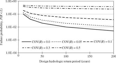
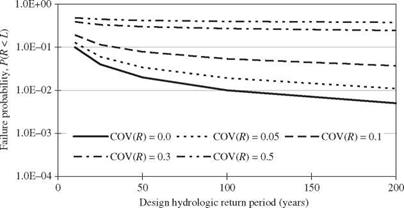
Figure 1.6 shows the effect of hydraulic uncertainty on the overall failure probability under the assumption that both random load and resistance are independent log-normal random variables. The figure can be produced eas­ily from the basic properties of log-normal random variables (see Sec. 2.6.2). Figure 1.6 clearly shows that by considering only inherent randomness of hydrologic load [the bottom curve corresponding to the coefficient of variation (COV), COV(R) = 0], the annual failure probability is significantly underesti­mated as the uncertainty of resistance COV(R) increases. As shown in Fig. 1.1, the inherent natural randomness of hydrologic processes is only one of the many uncertainties in hydrosystems engineering design. This figure clearly demonstrates the deficiency of the conventional frequency-analysis approach in reliability assessment of hydrosystems.

The basic idea of reliability engineering is to determine the failure probability of an engineering system, from which the safety of the system can be assessed or a rational decision can be made on the design, operation, or forecasting of the system, as depicted in Fig. 1.3. For example, Fig. 1.4 schematically illus­trates using reliability analysis for risk-based least-cost design of engineering infrastructures.

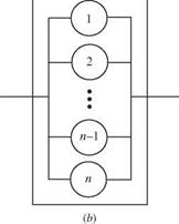
An infrastructure is a functioning system formed from a combination of a number of components. From the perspective of reliability analysis, infras­tructure systems can be classified in several ways. First, they can be grouped according to the sequential layout of the components (Fig. 1.5). A series sys­tem is a system of components connected in sequence along a single path, i. e., in series. Failure of any one of the components leads to failure of the entire system. A parallel system is one with its components connected side by side,

i. e., in parallel paths. Many engineering systems have built-in redundancy such that they function as a parallel system. Failure occurs when none of the parallel alternative paths function. Second, from the view point of the time consistency of the statistical characteristics of the systems, they can be classified as a time – invariant statistically stationary system (or static system) and a time-varying statistically nonstationary system (or dynamic system).

Infrastructures may follow different paths to failure. The ideal and simplest type is the case that the resistance and loading of the system are statistically independent of time, or a stationary system. Most of the existing reliability analysis methods have been developed for such a case.

A more complicated but realistic case is that for which the statistical char­acteristics of the loading or resistance or both are changing with time, e. g., floods from a watershed under urbanization, rainfall under the effect of global

D

E Q

D

00 2

D

♦ D

Figure 1.4 Risk-based least-cost design of infrastructural sys­tems. (After Yen and Tung, 1993.)

warming, sewer or water supply pipes with deposition, and fatigue or elastic behavior of steel structure members. This case can further be subdivided into the subcases of (1) the changing process is irreversible and accumulative and (2) the changing process is reversible, e. g., repairable. For some infrastructures, the statistical characteristics of the system change with space or in time (or both), e. g., a reach of highway or levee along different terrains. There are other subsets ofthese time-varying or space-varying dynamic failure cases. One is the subcase that a component of the system already has malfunctioned, but failure has not occurred because the loading has not yet reached the level of such failure, or there is a redundant component to take the load, but the strength of the system is weakened. Another subcase is changing the tolerance of failure, such as changing acceptable standards by regulations.