Category Hydrosystems Engineering Reliability Assessment and Risk Analysis

Limitations of Hydrologic Frequency Analysis

3.9.1 Distribution Selection: Practical Considerations

Many different probability distributions have been proposed for application to hydrologic data. Some of them were proposed because the underlying concept of the distribution matched the goal of hydrologic frequency analysis. For ex­ample, the extremal distributions discussed in Sec. 2.6.4 have very favorable properties for hydrologic frequency analysis. Ang and Tang (1984, p. 206) noted that the asymptotic distributions of extremes in several cases tend to converge on certain limiting forms for large sample sizes n, specifically to the double­exponential form or to two single-exponential forms. The extreme value from an initial distribution with an exponentially decaying tail (in the direction of the extreme) will converge asymptotically to the extreme-value type I (Gumbel) distribution form. Distributions with such exponentially decaying tails include the normal distribution and many others listed in Sec. 2.6. This is why Gumbel (1941) first proposed this distribution for floods, and it has gained consider­able popularity since then. Also, the properties of the central limit theorem discussed in Sec. 2.6.2 have made the lognormal distribution a popular choice for hydrologic frequency analysis.

In the 1960s, as the number of different approaches to flood frequency analy­sis were growing, a working group of U. S. government agency hydrologic experts was formed by the U. S. Water Resources Council to evaluate the best/preferred approach to flood frequency analysis. Benson (1968) reviewed the results of this working group and listed the following key results of their study:

1. There is no physical rule that requires the use of any specific distribution in the analysis of hydrologic data.

2. Intuitively, there is no reason to expect that a single distribution will apply to all streams worldwide.

3. No single method of testing the computed results against the original data was acceptable to all those on the working group, and the statistical consul­tants could not offer a mathematically rigorous method.

Subsequent to this study, the U. S. Water Resources Council (1967) recom­mended use of the log-Pearson type 3 distribution for all flood frequency anal­yses in the United States, and this has become the official distribution for all flood frequency studies in the United States. There are no physical arguments for the application of this distribution to hydrologic data. It has added flexi­bility over two-parameter distributions (e. g., Gumbel, lognormal) because the skewness coefficient is a third independent parameter, and the use of three parameters generally results in a better fit of the data. However, a number of researchers have suggested that the use of data for a single site may be insufficient to estimate the skewness coefficient properly.

Beard (1962) recommended that only average regional skewness coefficients should be applied in flood frequency analysis for a single station unless that record exceeds 100 years. This led the U. S. Water Resources Council (1967) to develop maps of regional skewness coefficient values that are averaged with the at-a-site skewness coefficient as a function of the number of years of record. For details on the procedure, see Interagency Advisory Committee on Water Data (1982). Linsley et al. (1982) noted that although regional skewness coefficients may not make for more reliable analysis, their use does lead to more consistency between values for various streams in the region.

With a Frequency Relation

Consider Example 3.2 in which the annual maximum flood peak discharges over a 15-year period on the Boneyard Creek at Urbana, Illinois, were analyzed. Suppose that the annual maximum floods follow the Gumbel distribution. The estimated 25-year flood peak discharge is 656 ft3/s. It is not difficult to imag­ine that if one had a second set of 15 years of record, the estimated 25-year flood based on the second 15-year record likely would be different from the first 15-year record. Also, combining with the second 15 years of record, the esti­mated 25-year flood magnitude based on a total of 30 years of record again would not have the same value as 656 ft3/s. This indicates that the estimated 25-year flood is subject to uncertainty that is due primarily to the use of lim­ited amount of data in frequency analysis. Furthermore, it is intuitive that the reliability of the estimated 25-year flood, based on a 30-year record, is higher than that based on a 15-year record.

From the preceding discussions one can conclude that using a limited amount of data in frequency analysis, the estimated value of a geophysical quantity of a particular return period xT and the derived frequency relation are subject to uncertainty. The degree of uncertainty of the estimated xT depends on the sample size, the extent of data extrapolation (i. e., return period relative to the record length), and the underlying probability distribution from which the data are sampled (i. e., the distribution). Since the estimated design quantity is subject to uncertainty, it is prudent for an engineer to quantify the magnitude of such uncertainty and assess its implications on the engineering design (Tung and Yen, 2005, Sec. 1.5). Further, Benson (1968) noted that the results oftheU. S. Water Resources Council study to determine the “best” distribution indicated that confidence limits always should be computed for flood frequency analysis.

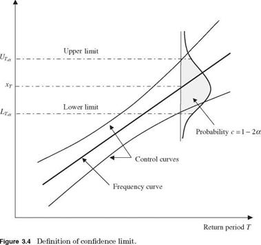
In practice, there are two ways to express the degree of uncertainty of a statis­tical quantity, namely, standard error and confidence interval (confidence limit). Because the estimated geophysical quantities of a particular return period are subject to uncertainty, they can be treated as a random variable associated with a distribution, as shown in Fig. 3.4. Similar to the standard deviation of a

Variate x

With a Frequency Relation


random variable, the standard error of estimate se measures the standard de­viation of an estimated statistical quantity from a sample, such as XT, about the true but unknown event magnitude. On the other hand, the confidence limit of an estimated quantity is an interval that has a specified probability (or confidence) to include the true value.

In the context of frequency analysis, the standard error of XT is a function of the distribution of the data series under consideration and the method of determining the distribution parameters. For example, the asymptotic (that is, as n ^ <x>) standard error of a T-year event se(XT) from a normal distribution can be calculated as (Kite, 1988)

f 2 + zT V/2

se (Xt ) = 2nT sx (3.21)

in which zT is the standard normal variate corresponding to the exceedance probability of 1/T, that is, Ф^т) = 1 – 1/T, n is the sample size, and sx is the sample standard deviation of random variable X. From the Gumbel distribu­tion, the standard error of XT is

Подпись: se(%T )Подпись: (3.22)Г 1 1 1/2

1 + 1.1396 Kt + 1.1 KT sx

n

To construct the confidence interval for XT or for the frequency curve, a con­fidence level c that specifies the desired probability that the specified range will include the unknown true value is predetermined by the engineer. In practice, a confidence level of 95 or 90 percent is used. Corresponding to the confidence level c, the significance level a is defined as a = 1 – c; for example, if the desired confidence level c = 90 percent, the corresponding significance level a = 10 percent. In determining the confidence interval, the common practice is to distribute the significance level a equally on both ends of the distribu­tion describing the uncertainty feature of estimated xT (see Fig. 3.4). In doing so, the boundaries of the confidence interval, called confidence limits, are de­fined. Assuming normality for the asymptotic sample distribution for XT, the approximated 100(1 – a) percent confidence interval for XT is

XT, a = XT – Z1-a/2 X Se(Xt) Xy, a = Xt + Z1-a/2 X Se(Xt) (3.23)

in which XT, a and XU, a are, respectively, the values defining the lower and up­per bounds for the 100(1 – a) percent confidence interval, and z1-a/2 = Ф-1 (1 – a/2). The confidence interval defined by Eq. (3.23) is only approximate and the approximation accuracy increases with sample size.

Similar to the frequency-factor method, the formulas to compute the upper and lower limits of confidence interval for XT has the same form as Eq. (3.6), except that the frequency-factor term is adjusted as

XT, a = X + KTl a X Sx X%a = X + K% a X Sx (3.24)

Подпись: KT,a = ZT ,a/2 With a Frequency Relation Подпись: (3.25)

in which K^ a and KU, a are the confidence-limit factors for the lower and upper limits of the 100(1 – a) percent confidence interval, respectively. For random samples from a normal distribution, the exact confidence-limit factors can be determined using the noncentral-t variates Z (Table 3.5). An approximation for K! p a with reasonable accuracy for n > 15 and a = 1 – c > 5 percent (Chowdhury et al., 1991) is

To compute KU, a, by symmetry, one only has to change za/2 by z1-a/2 inEq. (3.25). As was the case for Eq. (3.20), the confidence intervals defined by Eqs. (3.24) and (3.25) are most appropriate for samples from populations following a nor­mal distribution, and for nonnormal populations, these confidence limits are only approximate, with the approximation accuracy increasing with sample size.

For Pearson type 3 distributions, the values of confidence-limit factors for different return periods and confidence levels given in Eq. (3.24) can be mod­ified by introducing the scaling factor obtained from a first-order asymptotic

Подпись: 132
TABLE 3.5 95 Percent Confidence-Limit Factors for Normal Distribution

Return period (years)

n 2 5 10 25 50 100

KL KT, a

Ku KT, a

KL KT, a

Ku

KT, a

KL KT, a

Ku

KT, a

KL KT, a

Ku

KT, a

KL KT, a

Ku

KT, a

KL KT, a

Ku

KT, a

15

-0.4468

0.4468

0.3992

1.4641

0.7908

2.0464

1.1879

2.6880

1.4373

3.1095

1.6584

3.4919

20

-0.3816

0.3816

0.4544

1.3579

0.8495

1.9101

1.2535

2.5162

1.5085

2.9139

1.7351

3.2743

25

-0.3387

0.3387

0.4925

1.2913

0.8905

1.8257

1.2997

2.4109

1.5586

2.7942

1.7891

3.1415

30

-0.3076

0.3076

0.5209

1.2447

0.9213

1.7672

1.3345

2.3382

1.5965

2.7120

1.8300

3.0504

40

-0.2647

0.2647

0.5613

1.1824

0.9654

1.6898

1.3845

2.2427

1.6510

2.6041

1.8889

2.9310

50

-0.2359

0.2359

0.5892

1.1418

0.9961

1.6398

1.4194

2.1814

1.6892

2.5349

1.9302

2.8546

60

-0.2148

0.2148

0.6100

1.1127

1.0191

1.6042

1.4457

2.1378

1.7179

2.4859

1.9613

2.8006

70

-0.1986

0.1986

0.6263

1.0906

1.0371

1.5772

1.4664

2.1050

1.7406

2.4490

1.9858

2.7599

80

-0.1855

0.1855

0.6396

1.0730

1.0518

1.5559

1.4833

2.0791

1.7591

2.4199

2.0059

2.7279

90

-0.1747

0.1747

0.6506

1.0586

1.0641

1.5385

1.4974

2.0580

1.7746

2.3963

2.0226

2.7019

100

0.1656

0.1656

0.6599

1.0466

1.0746

1.5240

1.5095

2.0404

1.7878

2.3766

2.0370

2.6802

approximation of the Pearson type 3 to normal quantile variance ratio n as (Stedinger et al., 1983)

Kr, a = Kt + n(ZT,1-a/2 — Zt ) and Ky, a = Kt + n(ZT, a/2 — Zt ) (3.26)

Подпись: n = Подпись: 1 + yxKT + 1/2(1 + 3/iYx)KT + n var(yx)(ЭKT /дух)2 1 + (1/2)zT Подпись: (3.27)

where

Подпись: d KT dyx Подпись: 1 (4 — 1) With a Frequency Relation Подпись: (3.28)

in which yx is the estimated skewness coefficient, and

A simulation study by Whitley and Hromadka (1997) showed that the approx­imated formula for the Pearson type 3 distribution is relatively crude and that a better expression could be derived for more accurate confidence-interval de­termination.

Example 3.8 Referring to Example 3.3, determine the 95 percent confidence interval of the 100-year flood assuming that the sample data are from a lognormal distribution.

Solution In this case, with the 95 percent confidence interval c = 0.95, the corre­sponding significance level a = 0.05. Hence Z0.025 = Ф—1(0.025) = —1.960 and г0.975 = Ф—1(0.975) = +1.960. Computation of the 95 percent confidence interval associated with the selected return periods are shown in the table below. Column (4) lists the values ofthe upper tail ofthe standard normal quantiles associated with each return period, that is, Kt = zt = Ф—1(1 — 1/T). Since random floods are assumed to be lognormally distributed, columns (7) and (8) are factors computed by Eq. (3.25) for defining the lower and upper bounds of the 95 percent confidence interval of dif­ferent quantiles in log-space, according to Eq. (3.24), as

yT,0.95 = y + ZT,0.025 x sy yU,0.95 = y + ZT ,0.975 x sy

In the original space, the 95 percent confidence interval can be obtained simply by taking exponentiation as

ЧТ,0.95 = exp (уТ,0.95) and 3r,0.95 = exp (УТ,0.95)

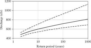
as shown in columns (11) and (12), respectively. The curves defining the 95 percent confidence interval, along with the estimated frequency curve, for a lognormal distri­bution are shown in Fig. 3.5.

95% CL for lognormal

With a Frequency Relation

Figure 3.5 95 percent confidence limits for a lognormal distri­bution applied to the annual maximum discharge for 1961­1975 on the Boneyard Creek at Urbana, IL.

Exceedance

Nonexceedance

Return period

probability

probability

T (years)

1 – p = 1/T

p = 1 – 1/ T

Kt = zt

УТ

qT

(1)

(2)

(3)

(4)

(5)

(6)

2

0.5

0.5

0.0000

6.165

475.9

5

0.2

0.8

0.8416

6.311

550.3

10

0.1

0.9

1.2816

6.386

593.7

25

0.04

0.96

1.7505

6.467

643.8

50

0.02

0.98

2.0537

6.520

678.3

100

0.01

0.99

2.3263

6.567

711.0

Return period

ZT,0.025

ZT,0.975

УТ,0.95

УТ,0.95

qT,0.95

qTU,0.95

T (years)

(7)

(8)

(9)

(10)

(11)

(12)

2

– 0 . 54

0.54

6.071

6.259

433.2

522.8

5

0.32

1.63

6.221

6.446

503.1

630.4

10

0.71

2.26

6.288

6.555

538.1

702.9

25

1.10

2.96

6.355

6.676

575.5

792.8

50

1.34

3.42

6.397

6.755

600.1

858.2

100

1.56

3.83

6.434

6.827

622.8

922.2

In order to define confidence limits properly for the Pearson type 3 distri­bution, the skewness coefficient must be estimated accurately, thus allowing the frequency factor KT to be considered a constant and not a statistic. Un­fortunately, with the Pearson type 3 distribution, no simple, explicit formula is available for the confidence limits. The Interagency Advisory Committee on Water Data (1982) (hereafter referred to as “the Committee”) proposed that the confidence limits for the log-Pearson type 3 distribution could be approxi­mated using a noncentral ^-distribution. The committee’s procedure is similar to that of Eqs. (3.24) and (3.25), except that KT, a and KU a, the confidence-limit factors for the lower and upper limits, are computed with the frequency factor KT replacing ZT in Eq. (3.25).

Example 3.9 Referring to Example 3.3, determine the 95 percent confidence intervals for the 2-, 10-, 25-, 50-, and 100-year floods assuming that the sample data are from a log-Pearson type 3 distribution.

Solution From Example 3.3, the mean and standard deviation of the logarithms of the peak flows were 6.17 and 0.173, and the number of data n is 15. For the 100-year flood, Kt is 1.8164, and for the 95 percent confidence limits, a is 0.05; thus Za/2 is -1.96. Thus KT a is -0.651, and the lower 95 percent confidence bound is 427.2 ft3/s. The upper and lower confidence bounds for all the desired flows are listed in the following table:

Return Period T (years)

Kt Eq. (3.8)

KT,0.025

Eq. (3.26)

KT,0.975 Eq. (3.26)

qT,0.95

(ft3/s)

au

4t,0.95 (ft3/s)

2

-0.0907

-0.6513

0.4411

427.2

516.1

10

1.0683

0.5260

1.9503

523.7

670.1

25

1.4248

0.8322

2.4705

552.2

733.2

50

1.6371

1.0082

2.7867

569.3

774.4

100

1.8164

1.1540

3.0565

583.8

811.4

Selection of Distribution Model

Based on a given sample of finite observations, procedures are needed to help identify the underlying distribution from which the random samples are drawn. Several statistical goodness-of-fit procedures have been developed (D’Agostino and Stephens, 1986). The insensitivity to the tail portion of the distribution of the conventional chi-square test and Kolmogorov-Smirnov test has been well known. Other more powerful goodness-of-fit criteria such as the probability plot correlation coefficient (Filliben, 1975) have been investigated and advocated (Vogel and McMartin, 1991). This and other criteria are described herein.

3.7.1 Probability plot correlation coefficients

Подпись: PPCC = Подпись: X^m=1(x(m) x)(ym y) [£ m=1( x(m) — x)2£ m=1( ym — y)2]0'5 Подпись: (3.17)

The probability plot is a graphic representation of the mth-order statistic of the sample x(m) as a function of a plotting-position F (x(m)). For each order statistic X(m), a plotting-position formula can be applied to estimate its corresponding nonexceedance probability F (X(m>), which, in turn, is used to compute the corre­sponding quantile Ym = G—1[F(X(m>)] according to the distribution model G( ) under consideration. Based on a sample with n observations, the probability plot correlation coefficient (PPCC) then can be defined mathematically as

where ym is the quantile value corresponding to F (x(m)) from a selected plotting – position formula and an assumed distribution model G(-), that is, ym = G-1 [F (x(m))]. It is intuitively understandable that if the samples to be tested are actually generated from the hypothesized distribution model G( ), the corre­sponding plot of X(m) versus ym would be close to linear. The values of F (x(m>) for calculating ym in Eq. (3.17) can be determined by using either a probability – or quantile-unbiased plotting-position formula. The hypothesized distribution model G( ) that yields the highest value of the PPCC should be chosen.

Critical values of the PPCCs associated with different levels of significance for various distributions have been developed. They include normal and lognormal distribution (Fillben, 1975; Looney and Gulledge, 1985; Vogel, 1986), Gumbel distribution (Vogel, 1986), uniform and Weibull distributions (Vogel and Kroll, 1989), generalized extreme-value distribution (Chowdhury et al., 1991), Pear­son type 3 distribution (Vogel and McMartin, 1991), and other distributions (D’Agostino and Stephens, 1986). A distribution is accepted as the underlying random mechanism with a specified significance level if the computed PPCC is larger than the critical value for that distribution.

3.7.2 Model reliability indices

Based on the observed (X(m>} and the computed {ym}, the degree of goodness of fit also can be measured by two reliability indices proposed by Leggett and Williams (1981). They are the geometric reliability index KG,

Подпись: KG =Подпись: 1 (ym/xjm)) 1 +( ym/x(m)) Подпись: 1 (ym/xjm)) 1 +( ym/x(m)) Selection of Distribution Model(3.18)

Подпись: KS = exp Selection of Distribution Model Selection of Distribution Model Подпись: (3.19)

and the statistical reliability index KS,

When the computed series {ym} perfectly matches with the observed sequence {x(m)}, the values of KG and KS reach their lower bound of 1.0. As the discrep­ancy between {x(m)} and {ym} increases, the values of KG and KS increase. Again, for each of KG and KS, two different values can be computed, each associated with the use of probability-unbiased and quantile-unbiased plotting-position formulas. The most suitable probability model is the one that is associated with the smallest value of the reliability index.

3.7.3 Moment-ratio diagrams

Relationships between product moments and the parameters of various distri­butions are shown in Table 3.4, which also can be found elsewhere (Patel et al., 1976; Stedinger et al., 1993). Similarly, the product-moment ratio diagram
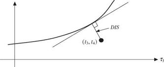
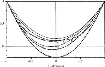
based on skewness coefficient and kurtosis (Stuart and Ord, 1987, p. 211) can be used to identify the distributions. When sample data are used, sample prod­uct moments are used to solve for the model parameters. However, owing to the low reliability of sample skewness coefficient and kurtosis, use of the product – moment ratio diagram for model identification is not reliable. Alternatively, the L-moment ratio diagram defined in the (r3, r4)-space (Fig. 3.3) also can be used for model identification. Namely, one can judge the closeness of the sam­ple L-skewness coefficient and L-kurtosis with respect to the theoretical r3 – r4 curve associated with different distribution models. Some types of distance mea­sures can be computed between the sample point of (t3, t4) and each theoretical т3 – t4 curve. One commonly used distance measure is to compute the shortest distance or distance in L-kurtosis direction fixed at the sample L-skewness coefficient (Pandey et al., 2001). Although it is computationally simple, the

Selection of Distribution Model

£


E Exponential G Gumbel L Logistic N Normal U Uniform


Generalized logistic _ _ Lower bound

Generalized extreme-value for wakeby Generalized pareto

Lognormal.. Lower bound for

Gamma all distributions


T4

Selection of Distribution Model

Figure 3.3 L-moment ratio diagram and shortest distance from a sample point.


Selection of Distribution Model

distance measure could not account for the sampling error in the sample L – skewness coefficient. To consider the effect of sampling errors in both the sam­ple L-skewness coefficient and L-kurtosis, the shortest distance between the sample point (t3, t4) and the theoretical r3 – r4 curve of each candidate distribu­tion model is computed for the measure of goodness of fit. The computation of the shortest distance requires locating a point on the theoretical т3 – t4 curve that minimizes the distance as

DIS = min J(t3 – T3)2 + [t4 – t4(t3)]2 (3.20)

T3

Since the theoretical t3 – t4 curve for a specified distribution is unique, determination of the shortest distance was accomplished by an appropriate one­dimensional search technique such as the golden-section procedure or others.

Example 3.7 (Goodness of Fit) Referring to the flood data given in Example 3.3, calculate the values of the probability-unbiased PPCCs and the two reliability indices with respect to the generalized Pareto distribution (GPA).

Solution Referring to Table 3.4, the GPA quantile can be obtained easily as

x(F) = § + в [1 – (1 – F )a]

a

According to the model parameter values obtained from Example 3.6, that is, a = 1.154, в = 361.36, § = 314.64, the GPA quantile can be computed as

x(F) = 314.64 + 36136 [1 – (1 – F)L154]

Using the probability-unbiased plotting position, i. e., the Weibull formula, the cor­responding GPA quantiles are calculated and shown in column (4) of the following table. From data in columns (2) and (4), the correlation coefficient can be obtained as 0.9843.

To calculate the two-model reliability indices, the ratios of GPA quantiles ym to the order flow q(m) are calculated in column (5) and are used in Eqs. (3.18) and (3.19) for Kg and Ks, respectively, as 1.035 and 1.015.

Rank (m) (1)

Ordered q(m) (2)

F (q(m)) = m/(n + 1) (3)

Ут

(4)

ym/q(m)

(5)

1

342

0.0625

337.1

0.985714

2

374

0.1250

359.4

0.960853

3

390

0.1875

381.4

0.977846

4

414

0.2500

403.1

0.973676

5

416

0.3125

424.6

1.020591

6

447

0.3750

445.7

0.997162

7

505

0.4375

466.6

0.923907

8

505

0.5000

487.1

0.964476

9

507

0.5625

507.2

1.000308

10

524

0.6250

526.8

1.005368

11

533

0.6875

546.0

1.024334

12

543

0.7500

564.5

1.039672

13

549

0.8125

582.4

1.060849

14

591

0.8750

599.4

1.014146

15

596

0.9375

615.0

1.031891

3.7.4 Summary

As the rule for selecting a single distribution model, the PPCC-based criterion would choose the model with highest values, whereas the other two criteria (i. e., reliability index and DIS) would select a distribution model with the smallest value. In practice, it is not uncommon to encounter a case where the values of the adopted goodness-of-fit criterion for different distributions are compatible, and selection of a best distribution may not necessarily be the best course of action, especially in the presence of sampling errors. The selection of acceptable distributions based on the their statistical plausibility through hypothesis test­ing, at the present stage, can only be done for the PPCCs for which extensive experiments have been done to define critical values under various significance levels (or type I errors) and different distributions.

Estimation of Distributional Parameters

For a chosen distributional model, its shape and position are completely defined by the associated parameters. By referring to Eq. (3.5), determination of the quantile also requires knowing the values of the parameters в.

There are several methods for estimating the parameters of a distribution model on the basis of available data. In frequency analysis, the commonly used parameter-estimation procedures are the method of maximum likelihood and the methods of moments (Kite, 1988; Haan, 1977). Other methods, such as method of maximum entropy (Li et al., 1986), have been applied.

3.6.1 Maximum-likelihood (ML) method

This method determines the values of parameters of a distribution model that maximizes the likelihood of the sample data at hand. For a sample of n indepen­dent random observations, x = (x1, x2,…, xn)1, from an identical distribution, that is,

Xi ~ fx(x | в) for i = 1,2,…, n

in which в = (0i, 02,…, 6m) a vector of m distribution model parameters, the likelihood of occurrence of the samples is equal to the joint probability

of {xi}i=1,2,…,n calculable by

n

L(x | в) = Ц fx(xi | в) (3.10)

i=1

in which L(x |в) is called the likelihood function. The ML method determines the distribution parameters by solving

Max L(x | в) = maxln[L(x | в)]

в в

or more specifically

nn

Подпись: (3.11)Maxll fx(Xi | в) = ln[fx(Xi | в)]

i=1 i=1

Estimation of Distributional Parameters
Подпись: Example 3.4 Referring to Eq. (2.79) for the exponential distribution as
Подпись: fx(x | в) = exp(-x/в)/в for x > 0, в > 0 determine the maximum likelihood estimate for в based on n independent random samples {xi }i=1,2,..., n Solution The log-likelihood function for the exponential distribution is

As can be seen, solving for distribution-model parameters by the ML principle is an unconstrained optimization problem. The unknown model parameters can be obtained by solving the following necessary conditions for the maximum:

Подпись: i=1

which is the sample mean.

Подпись: fx(x | а, в) = Подпись: 1 Подпись: _ 1 / x-а  2 PH в ) Подпись: for — 00 < x <00

Example 3.5 Consider a set of n independent samples, x = (xi, x%,…, xn)1, from a normal distribution with the following PDF:

Determine the ML estimators for the parameters a and в.

Подпись: L(x | а, в) = Estimation of Distributional Parameters Estimation of Distributional Parameters

Solution The likelihood function for the n independent normal samples is

Подпись:n, Y^n=1(xi – a)2

2в2

Estimation of Distributional Parameters Estimation of Distributional Parameters

Taking the partial derivatives of the preceding log-likelihood function with respect to a and в2 and setting them equal to zero results in

After some algebraic manipulations, one can easily obtain the ML estimates of normal distribution parameters a and в as

a Ei=1 xi в2 Ei=1(xi – a)2

aML = —n~ ^L =——————- n————

As can be seen, the ML estimation of the normal parameters for a is the sample mean and for в2 is a biased variance.

3.6.2 Product-moments-based method

By the moment-based parameter-estimation methods, parameters of a distribu­tion are related to the statistical moments of the random variable. The conven­tional method of moments uses the product moments of the random variable. Example 3.3 for frequency analysis is typical of this approach. When sample data are available, sample product moments are used to solve for the model parameters. The main concern with the use of product moments is that their reliabilities owing to sampling errors deteriorate rapidly as the order of moment
increases, especially when sample size is small (see Sec. 3.1), which is often the case in many geophysical applications. Hence, in practice only, the first few statistical moments are used. Relationships between product-moments and pa­rameters of distribution models commonly used in frequency analysis are listed in Table 3.4.

3.6.3 L-moments-based method

As described in Sec. 2.4.1, the L-moments are linear combinations of order statistics (Hosking, 1986). In theory, the estimators of L-moments are less sen­sitive to the presence of outliers in the sample and hence are more robust than the conventional product moments. Furthermore, estimators of L-moments are less biased and approach the asymptotic normal distributions more rapidly and closely. Hosking (1986) shows that parameter estimates from the L-moments are sometimes more accurate in small samples than are the maximum – likelihood estimates.

To calculate sample L-moments, one can refer to the probability-weighted moments as

вr = M1,r, o = E{X[Fx(X)]r} for r = 0,1,… (3.13)

which is defined on the basis of nonexceedance probability or CDF. The esti­mation of вг then is hinged on how Fx(X) is estimated on the basis of sample data.

Consider n independent samples arranged in ascending order as X(n) < X(n-1) < ■ ■ ■ < X(2) < X(1). The estimator for Fx(X(m>) for the mth – order statistic can use an appropriate plotting-position formula as shown in Table 3.2, that is,

m ___ a

F( X (m)) = 1———————- —— T for m = 1,2,…, n

n + 1 – b

with а > 0 and b > 0. The Weibull plotting-position formula (a = 0, b = 0) is a probability-unbiased estimator of Fx(X(m>). Hosking et al. (1985a, 1985b) show that a smaller mean square error in the quantile estimate can be achieved by using a biased plotting-position formula with a = 0.35 and b = 1. According to the definition of the в-moment вг in Eq. (3.13), its sample estimate br can be obtained easily as

1n

br = – J^X(m)[F (X(m))]r for Г = 0,1, … (3.14)

П i=1

Stedinger et al. (1993) recommend the use of the quantile-unbiased estimator of Fx(X(m)) for calculating the L-moment ratios in at-site and regional frequency analyses.

Distribution


Estimation of Distributional Parameters

Range


Product moments


L-Moments


*1 — M; *2 — O/

тз — 0;Т4 — 0.1226


Normal


— Ж < x < Ж


Min x — ln(Mx) x/2;

o2n x — ln(^2 +1);

Yx — 3^x +


2


1 /ln(x)-A1n x

2 V Oln x


Estimation of Distributional Parameters

Lognormal


x > 0


Eq. (2.68); Eq. (2.70)


*1 — % + aJ n / 2;

*2 — 2 а^ж(л/2 — 1) т3 — 0.1140; т4 — 0.1054


Estimation of Distributional Parameters

Rayleigh


% < x < Ж


a > 0

for в > 0: x > %; for в < 0: x < %


M — % + ав; о2 — ав2; Y — sign(в) JJS


Estimation of Distributional Parameters

Pearson 3


-(х—%)/в


*1 — в; *2 — в/2; тз — 1/3; Т4 — 1/6


Exponential fx(x) — e х/в/в


x > 0 m — в


M — % + 0.5772в; о2 — 2І6!; y — 1.1396


*1 — % + 0.5772в; *2 — в ln(2); т3 — 0.1699; т4 — 0.1504


Gumbel (EV1 fx(x) — 1 exp j — (xj^) — exp — (x^—^^ —ж < x < ж

for maxima)


M — вГ (1 + 1);

о2 — в2 [Г (l + D — г2(і + 1)]


*1 — % + вГ (1 +±);

*2 — в (1 — 2—1/рГ (1 + і)


fx (X) — a (XP)“ —1exP — ( ^


Weibull


а, в > 0; x > 0


*1 — % + (§) [1 — Г(1 + а)]; *2 — § (1 — 2—а )Г(1 + а);


а> 0: х < (% + §); а < 0: х > (% + І)


M — % + ) [1 — Г(1 + а)]; о2 — (в)2 [Г(1 + 2а) — Г2(1 + а)]


Generalized Fx (х) — exp| — (l — а{‘Х— %) ] 1/а|

extreme-value ^ *

(GEV)


2(1—3-°) 3.

(1—2—“) ’

1—5(4—“ )+10(3—“)—6(2—“)
1—2-“


тз

т4


Estimation of Distributional Parameters

а > 0:

z <х < (% +1); а < 0: Z < х < ж;


Generalized Fx (х) — 1 — (l — а (Х—%) ]1/а

Pareto (GPA)


Подпись: 123

For any distribution, the L-moments can be expressed in terms of the probability-weighted moments as shown in Eq. (2.28). To compute the sample L-moments, the sample probability-weighted moments can be obtained as

11 = 60

12 = 261 — 60

13 = 662 — 661 + 60 (3.15)

14 = 2063 — 3062 + 1261 — 60

Estimation of Distributional Parameters Подпись: t _ l3 t3 = І2 Подпись: t l4 t4 = І2 Подпись: (3.16)

where the lr s are sample estimates of the corresponding L-moments, the Xr s, respectively. Accordingly, the sample L-moment ratios can be computed as

where t2, t3, and t4 are the sample L-coefficient of variation, L-skewness co­efficient, and L-kurtosis, respectively. Relationships between L-moments and parameters of distribution models commonly used in frequency analysis are shown in the last column of Table 3.4.

Example 3.6 Referring to Example 3.3, estimate the parameters of a generalized Pareto (GPA) distribution by the L-moment method.

Solution Since the GPA is a three-parameter distribution, the calculation of the first three sample L-moments is shown in the following table:

Year

qi (ft3/s)

Ordered q(i) (ft3/s)

Rank

(i)

F (q(i)) =

(i — 0.35)/n

q(i) x F(q(i))

q(i) x F (q(i))2

q(i) x F (q(i))3

1961

390

342

1

0.0433

14.82

0.642

0.0278

1962

374

374

2

0.1100

41.14

4.525

0.4978

1963

342

390

3

0.1767

68.90

12.172

2.1504

1964

507

414

4

0.2433

100.74

24.513

5.9649

1965

596

416

5

0.3100

128.96

39.978

12.3931

1966

416

447

6

0.3767

168.37

63.419

23.8880

1967

533

505

7

0.4433

223.88

99.255

44.0030

1968

505

505

8

0.5100

257.55

131.351

66.9888

1969

549

507

9

0.5767

292.37

168.600

97.2260

1970

414

524

10

0.6433

337.11

216.872

139.5210

1971

524

533

11

0.7100

378.43

268.685

190.7666

1972

505

543

12

0.7767

421.73

327.544

254.3922

1973

447

549

13

0.8433

462.99

390.455

329.2836

1974

543

591

14

0.9100

537.81

489.407

445.3605

1975

591

596

15

0.9767

582.09

568.511

555.2459

Sum =

7236

4016.89

2805.930

2167.710

Note that the plotting-position formula used in the preceding calculation is that pro­posed by Hosking et al. (1985a) with a = 0.35 and b = 1.

Based on Eq. (3.14), the sample estimates of Pj, for j = 0,1, 2, 3, are Ьз = 428.4, b1 = 267.80, Ьз = 187.06, and b4 = 144.51. Hence, by Eq. (3.15), the sample estimates of к j, j = 1,2, 3,4, are I1 = 482.40, I2 = 53.19, I3 = -1.99, and I4 = 9.53, and the corresponding sample L-moment ratios Tj, for j = 2, 3, 4, are t2 = 0.110, t3 = —0.037, and t4 = 0.179.

Estimation of Distributional Parameters

By referring to Table 3.4, the preceding sample h = 482.40, I2 = 53.19, and t3 = —0.037 can be used in the corresponding L-moment and parameter relations, that is,

Analytical Approaches

Analytical Approaches Подпись: в Подпись: (3.5)

An alternative to the graphic technique is to estimate the statistical parameters of a distribution from the sample data (refer to Sec. 3.6). Then the distribution model can be used to solve for the variate value corresponding to any desired return period or probability as

in which F-1(e) is the inverse cumulative distribution function with the model parameter vector в. Equation (3.5) can be applied when the inverse distribu­tion function forms are analytically amenable, such as for the Gumbel, gener­alized extreme value, generalized logistic, and generalized Pareto distributions (see Sec. 2.6.6).

Example 3.2 Consider that the annual maximum floods follow a lognormal distribu­tion with a mean of 490 ft3/s and a standard deviation of 80 ft3/s. Determine the flood magnitude with a 1-in-100 chance of being exceeded in any given year.

Solution From Eqs. (2.67a) and (2.67b), the parameters of a lognormal distribution, for annual maximum flood Q, can be obtained as

Подпись: = 0.1622Obq = ^ln (vQ +[5]) = ^ln (490) + 1 Mnq = ln(MQ) – 1 Oj2n Q = ln(490) – 1(0.1622)2 = 6.1812

Since ln( Q) follows a normal distribution with a mean of mn q = 6.1812 and a stan­dard deviation of Oln q = 0.1622 as previously computed, the magnitude of the log – transformed 100-year flood can be calculated by

ln(g100)—= Ф-1 f 1 – -^ = Ф-1(0.99) = 2.34

Oln Q V 100 у

Hence ln(^100) = Mln Q + 2.34 x Olnq = 6.5607, and the corresponding 100-year flood magnitude can be calculated as дю0 = exp[ln(q10Q)] = 706.8 ft3/s.

For some distributions, such as Pearson type 3 or log-Pearson type 3, the appropriate probability paper or CDF inverse form is unavailable. In such a case, an analytical approach using the frequency factor KT is applied:

XT = l^x + Kt x ax (3.6)

in which xT is the variate corresponding to a return period of T, /гх and oX are the mean and standard deviation of the random variable, respectively, and KT is the frequency factor, which is a function of the return period T or P (X > xT) and higher moments, if required. It is clear that a plot of Eq. (3.6) (xT versus KT)
on linear graph paper will yield a straight line with slope of ax and intercept l^x at Kt = 0.

In order for Eq. (3.6) to be useful, the functional relationship between Kt and exceedance probability or return period must be determined for the distribution to be used. In fact, the frequency factor Kt = (xT — xx)/ax is identical to a standardized variate corresponding to the exceedance probability of 1/T for a particular distribution model under consideration. For example, if the normal distribution is considered, then Kt = zT = Ф—41 — T —:). The same applies to the lognormal distribution when the mean and standard deviation of log – transformed random variables are used. Hence the standard normal probability table (Table 2.2) provides values of the frequency factor for sample data from normal and log normal distributions. Once this relation is known, a nonlinear probability or return-period scale can be constructed to replace the linear Kt scale, and thus special graph paper can be constructed for any distribution so that plot of xT versus P or T will be linear.

Gumbel probability paper has been printed, although it is not readily avail­able from commercial sources. Referring to Eq. (2.85a), the relationship between Kt and T for this distribution can be derived as

Analytical Approaches

V6

n


T

T – 1


Kt


0.5772 + ln


(3.7)


Analytical Approaches

Подпись: KT (YX) = — Yx Подпись: 1 + ZT Подпись: Yx ~6 Подпись: Yx ~6 Подпись: 21 3 1 Подпись: (3.8)

For Pearson and log-Pearson type 3 distributions, linearization can be ac­complished according to Eq. (3.6). However, for this distribution, the frequency factor is a function of both P or T and the skewness coefficient yx. This means that a different nonlinear P or T scale is required for each skewness coeffi­cient, and therefore, it is impractical to construct a probability paper for this distribution. However, it should be pointed out that if yx = 0 in log-space, the log-Pearson type 3 reduces to the lognormal distribution, and thus commercial lognormal probability paper can be used. The relationship between frequency factor Kt, T, and yx cannot be developed in a closed form, as was done for the Gumbel distribution in Eq. (3.7). However, the relationship can be computed numerically, and the results are given in Table 3.3. For 0.99-1 < T < 100 and |yx | < 2, the frequency-factor values are well approximated by the Wilson – Hilferty transformation (Stedinger et al., 1993):

in which zT is the standard normal quantile with exceedance probability of 1/T.

The procedure for using the frequency-factor method is outlined as follows: 1

Return period in years

Skewness coefficient yx

2

5

10 25 50 Exceedence probability

100

200

0.50

0.20

0.10

0.04

0.02

0.01

0.005

3.0

-0.396

0.420

1.180

2.278

3.152

4.051

4.970

2.9

-0.390

0.440

1.195

2.277

3.134

4.013

4.909

2.8

-0.384

0.460

1.210

2.275

3.114

3.973

4.847

2.7

-0.376

0.479

1.224

2.272

3.093

3.932

4.783

2.6

-0.368

0.499

1.238

2.267

3.071

3.889

4.718

2.5

-0.360

0.518

1.250

2.262

3.048

3.845

4.652

2.4

-0.351

0.537

1.262

2.256

3.023

3.800

4.584

2.3

-0.341

0.555

1.274

2.248

2.997

3.753

4.515

2.2

-0.330

0.574

1.284

2.240

2.970

3.705

4.444

2.1

-0.319

0.592

1.294

2.230

2.942

3.656

4.372

2.0

-0.307

0.609

1.302

2.219

2.912

3.605

4.298

1.9

-0.294

0.627

1.310

2.207

2.881

3.553

4.223

1.8

-0.282

0.643

1.318

2.193

2.848

3.499

4.147

1.7

-0.268

0.660

1.324

2.179

2.815

3.444

4.069

1.6

-0.254

0.675

1.329

2.163

2.780

3.388

3.990

1.5

-0.240

0.690

1.333

2.146

2.743

3.330

3.910

1.4

-0.225

0.705

1.337

2.128

2.706

3.271

3.828

1.3

-0.210

0.719

1.339

2.108

2.666

3.211

3.745

1.2

-0.195

0.732

1.340

2.087

2.626

3.149

3.661

1.1

-0.180

0.745

1.341

2.066

2.585

3.087

3.575

1.0

-0.164

0.758

1.340

2.043

2.542

3.022

3.489

0.9

-0.148

0.769

1.339

2.018

2.498

2.957

3.401

0.8

-0.132

0.780

1.336

1.993

2.453

2.891

3.312

0.7

-0.116

0.790

1.333

1.967

2.407

2.824

3.223

0.6

-0.099

0.800

1.328

1.939

2.359

2.755

3.132

0.5

-0.083

0.808

1.323

1.910

2.311

2.686

3.041

0.4

-0.066

0.816

1.317

1.880

2.261

2.615

2.949

0.3

-0.050

0.824

1.309

1.849

2.211

2.544

2.856

0.2

-0.033

0.830

1.301

1.818

2.159

2.472

2.763

0.1

-0.017

0.836

1.292

1.785

2.107

2.400

2.670

0.0

0

0.842

1.282

1.751

2.054

2.326

2.576

-0.1

0.017

0.846

1.270

1.716

2.000

2.252

2.482

-0.2

0.033

0.850

1.258

1.680

1.945

2.178

2.388

-0.3

0.050

0.853

1.245

1.643

1.890

2.104

2.294

-0.4

0.066

0.855

1.231

1.606

1.834

2.029

2.201

-0.5

0.083

0.856

1.216

1.567

1.777

1.955

2.108

-0.6

0.099

0.857

1.200

1.528

1.720

1.880

2.016

-0.7

0.116

0.857

1.183

1.488

1.663

1.806

1.926

-0.8

0.132

0.856

1.166

1.448

1.606

1.733

1.837

-0.9

0.148

0.854

1.147

1.407

1.549

1.660

1.749

-1.0

0.164

0.852

1.128

1.366

1.492

1.588

1.664

-1.1

0.180

0.848

1.107

1.324

1.435

1.518

1.581

-1.2

0.195

0.844

1.086

1.282

1.379

1.449

1.501

-1.3

0.210

0.838

1.064

1.240

1.324

1.383

1.424

-1.4

0.225

0.832

1.041

1.198

1.270

1.318

1.351

-1.5

0.240

0.825

1.018

1.157

1.217

1.256

1.282

-1.6

0.254

0.817

0.994

1.116

1.166

1.197

1.216

Return period in years

Skewness coefficient yx

2

5

10 25 50 Exceedence probability

100

200

0.50

0.20

0.10

0.04

0.02

0.01

0.005

-1.7

0.268

0.808

0.970

1.075

1.116

1.140

1.155

-1.8

0.282

0.799

0.945

1.035

1.069

1.087

1.097

-1.9

0.294

0.788

0.920

0.996

1.023

1.037

1.044

-2.0

0.307

0.777

0.895

0.959

0.980

0.990

0.995

-2.1

0.319

0.765

0.869

0.923

0.939

0.946

0.949

-2.2

0.330

0.752

0.844

0.888

0.900

0.905

0.907

-2.3

0.341

0.739

0.819

0.855

0.864

0.867

0.869

-2.4

0.351

0.725

0.795

0.823

0.830

0.832

0.833

-2.5

0.360

0.711

0.771

0.793

0.798

0.799

0.800

-2.6

0.368

0.696

0.747

0.764

0.768

0.769

0.769

-2.7

0.376

0.681

0.724

0.738

0.740

0.740

0.741

-2.8

0.384

0.666

0.702

0.712

0.714

0.714

0.714

-2.9

0.390

0.651

0.681

0.683

0.689

0.690

0.690

-3.0

0.396

0.636

0.666

0.666

0.666

0.667

0.667

SOURCE: U. S. Water Resources Council (1981).

2. For the desired return period, determine the associated value of KT for the distribution.

3. Compute the desired quantile value using Eq. (3.6) with x replacing цx and sx replacing ax, that is,

XT = x + KT x sx (3.9)

It should be recognized that the basic difference between the graphic and analytical approaches is that each represents a different method of estimating the statistical parameters of the distribution being used. By the analytical ap­proach, a best-fit line is constructed that then sets the statistical parameters. In the mathematical approach, the statistical parameters are first computed from the sample, and effectively, the line thus determined is used. The line deter­mined using the mathematical approach is in general a poorer fit to the observed data than that obtained using the graphic approach, especially if curve-fitting procedures are applied. However, the U. S. Water Resources Council (1967) rec­ommended use of the mathematical approach because

1. Graphic least-squares methods are avoided to reduce the incorporation of the random characteristics of the particular data set (especially in the light of the difficulty in selecting the proper plotting-position formula).

2. The generally larger variance of the mathematical approach is believed to help compensate for the typically small data sets.

Example 3.3 Using the frequency-factor method, estimate the flows with return pe­riods of 2, 10, 25, 50, and 100 years for the Boneyard Creek using the Gumbel and log-Pearson type 3 distributions. Use the historical data in Example 3.1 as a basis for the calculations.

Solution Based on the samples, the method requires determination of the frequency factor Kt in

xt = x + Kt x sx

Analytical Approaches
Подпись: (6361.8)1/2 = 79.8ft3/s

For the Gumbel distribution, values of Kt can be calculated by Eq. (3.7). For the log-Pearson type 3 distribution, Table 3.3 or Eq. (3.8) can be used, which requires computation of the skewness coefficient. The calculations of relevant sample moments are shown in the following table:

Year

Original scale

Log – Transformed scale

gi (ft3/s)

gi2

gi3

Уі = ln( gi)

Уі2

Уі3

1961

390

1.52e + 05

5.93e + 07

5.97

35.59

212.36

1962

374

1.40e + 05

5.23e + 07

5.92

35.10

207.92

1963

342

1.17e + 05

4.00e + 07

5.83

34.05

198.65

1964

507

2.57e + 05

1.30e + 08

6.23

38.79

241.63

1965

596

3.55e + 05

2.12e + 08

6.39

40.84

260.95

1966

416

1.73e + 05

7.20e + 07

6.03

36.37

219.33

1967

533

2.84e + 05

1.51e + 08

6.28

39.42

247.50

1968

505

2.55e + 05

1.29e + 08

6.22

38.75

241.17

1969

549

3.01e + 05

1.65e + 08

6.31

39.79

251.01

1970

414

1.71e + 05

7.10e + 07

6.03

36.31

218.81

1971

524

2.75e + 05

1.44e + 08

6.26

39.21

245.49

1972

505

2.55e + 05

1.29e + 08

6.22

38.75

241.17

1973

447

2.00e + 05

8.93e + 07

6.10

37.24

227.27

1974

543

2.95e + 05

1.60e + 08

6.30

39.65

249.70

1975

591

3.49e + 05

2.06e + 08

6.38

40.73

259.92

Sum =

7236

3.58e + 06

1.81e + 09

92.48

570.58

3522.88

For the Gumbel distribution,

For the log-Pearson type 3 distribution,

Eln(gf) 92.48


6.165


У =

n

15

sy =

1—1 1

1 1

gy =

n

m3

(n – 1)(n – 2) syj


= (0.417/14)1/2 = 0.173


15(-0.00336) (14)(13)(0.173)3


-0.540


in which m3 = Уз — Уі + 2ny3. The determination of the values of frequency

factor corresponding to different return periods is shown in the following table:

Frequency factor by distribution

Return period

Exceedance

Nonexceedance

Gumbel

LP3

(years)

probability

probability

Eq. (3.7)

Eq. (3.8)

2

0.50

0.50

—0.1643

0.0892

10

0.10

0.90

1.3046

1.2093

25

0.04

0.96

2.0438

1.5526

50

0.02

0.98

2.5923

1.7570

100

0.01

0.99

3.1367

1.9292

Based on the preceding frequency-factor values, the flood magnitude of the various

return periods

can be determined as

Frequency curves

by distribution (ft3/s)

Return period

Gumbel

LP3

(years)

qT = 482.4 + 79.8Kt, EV1

qT = exp(6.165 + 0.173Kt, LP3)

2

469.3

483.3

10

586.5

586.4

25

645.4

622.2

50

689.2

644.5

100

732.6

663.9

One could compare these results for the Gumbel distribution with those obtained from the graphic approach of Example 3.1.

Graphic Approach

Once the data series is identified and ranked and the plotting position is calcu­lated, a graph of magnitude x versus probability [P(X > x), P(X < x), or T] can be plotted and a distribution fitted graphically. To facilitate this procedure, it is common to use some specially designed probability graph paper rather than linear graph paper. The probability scale in those special papers is chosen such that the resulting probability plot is a straight line. By plotting the data using a particular probability scale and constructing a best-fit straight line through the data, a graphic fit is made to the distribution used in constructing the prob­ability scale. This is a graphic approach to estimate the statistical parameters of the distribution.

Example 3.1 illustrates the graphic approach to the analysis of flood data. The general procedure is as follows: [2] [3] 3 [4]

5. Extend the line to the highest return-period value needed, and read all re­quired return-period values off the line.

Example 3.1 The Boneyard Creek stream gauging station was located near the fire station on the campus of the University of Illinois at Urbana-Champaign. From the USGS Water Supply Papers, the partial duration data of peak discharges above 400 ft3/s between the water years 1961 and 1975 were obtained and listed below. In addi­tion, for the years when there was no flow in a year exceeding 400 ft3/s, the peak flow for that year is given in parenthesis (e. g., 1961).

Year

Discharge, ft3/s

Year

Discharge, ft3 /s

1961

(390)

1969

549, 454

1962

(374)

1970

414, 410

1963

(342)

1971

434, 524

1964

507

1972

505, 415, 406

1965

579, 406, 596

1973

428, 447, 407

1966

416

1974

468, 543, 441

1967

533

1975

591, 497

1968

505

(a) List the ranked annual maximum series. Also compute and list the corresponding plotting positions (return period) and exceedance probability P (X > x).

(b) Plot the annual maximum series on (i) Gumbel paper and (ii) lognormal paper.

(c) Construct a best-fit line through the nonlinear plots, and estimate the flows for return periods of 2, 10, 25, and 50 years.

Solution n = 15 (a)

Annual Maximum Discharge (ft3/s)

Rank

(m)

‘T _ n+1 Tm = m

(years)

P(X > X(m))

= 1/Tm

P (X < x(m))

= 1 – 1/Tm

596

1

16.00

0.0625

0.9375

591

2

8.00

0.1250

0.8750

549

3

5.33

0.1875

0.8125

543

4

4.00

0.2500

0.7500

533

5

3.20

0.3125

0.6875

524

6

2.67

0.3750

0.6250

507

7

2.29

0.4375

0.5625

505

8

2.00

0.5000

0.5000

505

9

1.78

0.5625

0.4375

447

10

1.60

0.6250

0.3750

416

11

1.46

0.6875

0.3125

414

12

1.33

0.7500

0.2500

390

13

1.23

0.8125

0.1875

374

14

1.14

0.8750

0.1250

342

15

1.06

0.9375

0.0625

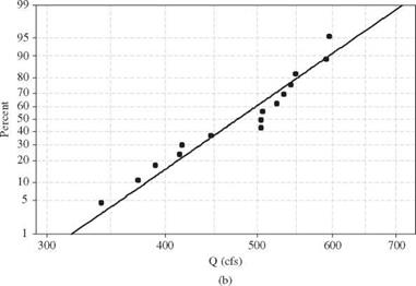
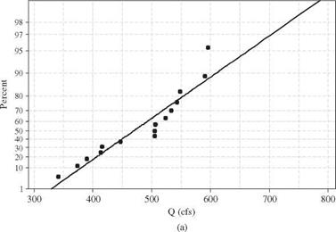
(b) Plots of the annual maximum flow series on the Gumbel and lognormal probability papers are shown in Fig. 3.2.

Graphic Approach

Graphic Approach

Figure 3.2 Probability plot for the annual maximum series for 1961-1975 on the Boneyard Creek at Urbana, IL: (a) Gumbel probability plot; (b) lognormal probability plot.


(c) The following table summarizes the results read from the plots:


Return Period (years)

Distribution

2

10

25

50

Gumbel

470

610

680

730

Lognormal

475

590

650

700


Graphic Approach

Probability Estimates for Data Series: Plotting Positions (Rank-order Probability)

As stated previously, the objective of frequency analysis is to fit geophysical data to a probability distribution so that a relationship between the event magnitude and its exceedance probability can be established. The first step in the procedure is to determine the type of data series (i. e., event magnitude) to be used. In order to fit a probability distribution to the data series, estimates of probability (or equivalent return period) must be assigned to each magnitude in the data series.

Consider a data series consisting of the entire population of N values for a particular variable. If this series were ranked according to decreasing magni­tude, it could be stated that the probability of the largest variate being equaled or exceeded is 1/N, where N is the total number of variates. Similarly, the exceedance probability of the second largest variate is 2/N, and so forth. In general,

1 m

P(X > X(m)) = — = – (3.2)

in which m is the rank of the data in descending order, x—) is the mth largest variate in a data series of size N, and Tm is the return period associated with x—). In practice, the entire population is not used or available. However, the reasoning leading to Eq. (3.2) is still valid, except that the result is now only an estimate of the exceedance probability based on a sample. Equation (3.2), which shows the ranked-order probability, is called a plotting position formula because it provides an estimate of probability so that the data series can be plotted (magnitudes versus probability).

Equation (3.2) is appropriate for data series from the population. Some mod­ifications are made to avoid theoretical inconsistency when it is applied to sam­ple data series. For example, Eq. (3.2) yields an exceedance probability of 1.0 for the smallest variate, implying that all values must be equal or larger. Since only
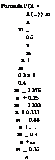
a sample is used, there is a likelihood that at some future time an event with a lower value could occur. In application, if the lower values in the series are not of great interest, this weakness can be overlooked, and in fact, Eq. (3.2) is used in the analysis of the annual exceedance series. A number of plotting-position formulas have been introduced that can be expressed in a general form as

1 m — a

P(x > x(m)) = um = — = n + 1 _ b (3.[1]

in which a > 0 and b > 0 are constants, and n is the number of observations in the sample data series. Table 3.2 lists several plotting-position formulas that have been developed and used in frequency analysis. Perhaps the most popular plotting-position formula is the Weibull formula (with a = 0 and b = 0):

1 m

P{X > X(m)) = Um = ^ = ^^ (3.4)

Tm n + 1

As shown in Table 3.2, it is noted that although these formulas give different results for the highest values in the series, they yield very similar results for the middle to lowest values, as seen in the last two columns.

Plotting-position formulas in the form of Eq. (3.3) can be categorized into being probability-unbiased and quantile-unbiased. The probability-unbiased

Probability Estimates for Data Series: Plotting Positions (Rank-order Probability) Подпись: 1 P (X > x(m)) Подпись: for n = 20

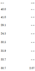
Подпись: m = 1Подпись: m = 10Подпись: 20.0 2.00 40.0 2.11 41.0 2.10 29.1 2.10 24.5 2.10 30.5 2.10 35.9 2.10 33.7 2.10 30.7 2.07

Подпись: Name California (1923) Hazen (1930) Weibull (1939) Leivikov (1955) Blom (1958) Tukey (1962) Gringorten (1963) Cunnane (1978) Hosking et al. (1985) Подпись: Formula P(X > X(m)) m n m _ 0.5 n m n + 1 m _ 0.3 n + 0.4 m _ 0.375 n + 0.25 m _ 0.333 n + 0.333 m _ 0.44 n + 0.12 m _ 0.4 n + 0.2 m _ 0.35 n

TABLE 3.2 Plotting-Position Formulas

plotting-position formula is concerned with finding a probability estimate u(m) for the exceedance probability of the mth largest observation such that E[G(X(m))] = u(m), in which G(X(m>) = P(X > X(m>). In other words, the probability-unbiased plotting position yields the average exceedance probabil­ity for the mth largest observation in a sample of size n. If the data are indepen­dent random samples regardless of the underlying distribution, the estimator U(m) = G(X (m)) will have a beta distribution with the mean E (U(m)) = m/(n+l). Hence the Weibull plotting-position formula is probability-unbiased. On the other hand, Cunnane (1978) proposed quantile-unbiased plotting positions such that average value of the mth largest observation should be equal to G-1(u(m>), that is, E(X(m)) = G-1(u(m)). The quantile-unbiased plotting-position formula, however, depends on the assumed distribution G( ). For example, referring to Table 3.2, the Blom plotting-position formula gives nearly unbiased quantiles for the normal distribution, and the Gringorton formula gives nearly unbiased quantiles for the Gumbel distribution. Cunnane’s formula, however, produces nearly quantile-unbiased plotting positions for a range of distributions.

Return Period

Return Period Подпись: 1 1 - P (X < xT) Подпись: (3.1)

Hydrosystems engineers have been using the concept of the return period (or sometimes called recurrence interval) as a substitute for probability because it gives some physical interpretation to the probability. The return period for a given event is defined as the period of time on the long-term average at which a given event is equaled or exceeded. Hence, on average, an event with a 2-year return period will be equaled or exceeded once in 2 years. The relation­ship between the probability and return period is given by

in which xT is the value of the variate corresponding to a T-year return period. For example, if the probability that a flood will be equaled or exceeded in a single year is 0.1, that is, P (X > xT) = 0.1, the corresponding return period is 1/P (X > xT) = 1/0.1 = 10 years. Note that P (X > xT) must be the probabil­ity that the event is equaled or exceeded in any one year and is the same for each year regardless of the magnitudes that occurred in prior years. This is so because the events are independent, and the long-term probabilities are used without regard to the order in which they may occur. A common error or mis­conception is to assume, for example, that if the 100-year event occurs this year, it will not occur again for the next 100 years. In fact, it could occur again next year and then not be repeated for several hundred years. This misconception resulted in considerable public complaints when the Phoenix area experienced two 50-year and one 100-year floods in a span of 18 months in 1978-1979 and the Milwaukee area experienced 100-year floods in June 1997 and June 1998.

Hence it is more appropriate and less confusing to use the odds ratio; e. g., the 100-year event can be described as the value having 1-in-100 chance being exceeded in any one year (Stedinger et al., 1993). In the United States in recent years it has become common practice to refer to the 100-year flood as the 1 per­cent chance exceedance flood, and similar percent chance exceedance descrip­tions are used for other flood magnitudes (U. S. Army Corps of Engineers, 1996).

The most common time unit for return period is the year, although semi­annual, monthly, or any other time period may be used. The time unit used to form the time series will be the unit assigned to the return period. Thus an annual series will have a return-period unit of years, and a monthly series will have return-period unit of months. However, one should be careful about compliance with the statistical independence assumption for the data series. Many geophysical data series exhibit serial correlation when the time interval is short, which can be dealt with properly only by time-series analysis procedures (Salas, 1993).

Types of Geophysical Data Series

The first step in the frequency-analysis process is to identify the set of data or sample to be studied. The sample is called a data series because many events of interest occur in a time sequence, and time is a useful frame of reference. The events are continuous, and thus their complete description as a function of time would constitute an infinite number of data points. To overcome this, it is customary to divide the events into a series of finite time increments and con­sider the average magnitude or instantaneous values of the largest or smallest within each interval. In frequency analysis, geophysical events that make up the data series generally are assumed to be statistically independent in time. In the United States, the water year concept was developed to facilitate the independence of hydrologic flood series. Throughout the eastern, southern, and Pacific western areas of the United States, the season of lowest stream flow is late summer and fall (August-October) (U. S. Department of Agriculture, 1955). Thus, by establishing the water year as October 1 to September 30, the chance of having related floods in each year is minimized, and the assumption of independence in the flood data is supported. In case time dependence is present in the data series and should be accounted for, procedures developed in time series analysis (Salas et al., 1980; Salas, 1993) should be applied. This means that the events themselves first must be identified in terms of a beginning and an end and then sampled using some criterion. Usually only one value from each event is included in the data series. There are three basic types of data series extractable from geophysical events:

1. A complete series, which includes all the available data on the magnitude of a phenomenon. A complete data series is used most frequently for flow – duration studies to determine the amount of firm power available in a pro­posed hydropower project or to study the low-flow behavior in water quality management. Such a data series is usually very large, and since in some in­stances engineers are only interested in the extremes of the distribution (e. g., floods, droughts, wind speeds, and wave heights), other data series often are more practical. For geophysical events, data in a complete series often exhibit significant time dependence, which makes the frequency-analysis procedure described herein inappropriate.

2. An extreme-value series is one that contains the largest (or smallest) data value for each of a number of equal time intervals. If, for example, the largest data value in each year of record is used, the extreme-value series is called an annual maximum series. If the smallest value is used, the series is called an annual minimum series.

3. A partial-duration series consists of all data above or below a base value. For example, one might consider only floods in a river with a magnitude greater than 1,000 m3/s. When the base value is selected so that the number of events included in the data series equals the number of years of record, the resulting series is called an annual exceedance series. This series contains the n largest or n smallest values in n years of record.

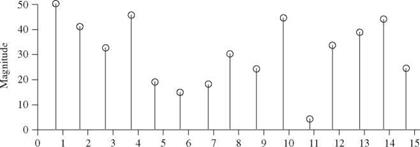
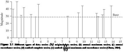
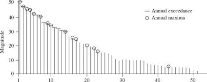
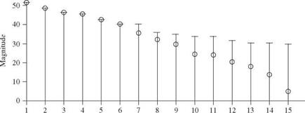
The selection of geophysical data series is illustrated in Fig. 3.1. Figure 3.1a represents the original data; the length of each line indicates the magnitude of the event. Figure 3.16 shows an annual maximum series with the largest data value in each year being retained for analysis. Figure 3.1c shows the data values that would be included in an annual exceedance series. Since there are 15 years of record, the 15 largest data values are retained. Figure 3.1d and e illustrate for comparison the rank in descending order of the magnitude of the events in each of the two series. As shown in Fig. 3.1d and e the annual maximum series and the annual exceedance series form different probability distributions, but when used to estimate extreme floods with return periods of 10 years or more, the differences between the results from the two series are minimal, and the annual maximum series is the one used most commonly. Thus this chapter focuses on the annual maximum series in the following discussion and examples.

Another issue related to the selection of the data series for frequency anal­ysis is the adequacy of the record length. Benson (1952) generated randomly

Types of Geophysical Data Series

Yr.


(a)


Types of Geophysical Data Series

Yr.


(b)


Types of Geophysical Data Series

Types of Geophysical Data Series

Rank

(d)

Types of Geophysical Data Series

Rank

(e)

Figure 3.1 (Continued) selected values from known probability distributions and determined the record length necessary to estimate various probability events with acceptable error levels of 10 and 25 percent. Benson’s results are listed in Table 3.1. Linsley et al. (1982, p. 358) reported that similar simulation-based studies at Stanford University found that 80 percent of the estimates of the 100-year flood based on 20 years of record were too high and that 45 percent of the overestimates

TABLE 3.1 Number of Years of Record Needed to Obtain Estimates of Specified Design Probability Events with Acceptable Errors of 10 and 25 Percent

Design probability

Return period (years)

10% error (years)

25% error (years)

0.1

10

90

18

0.02

50

110

39

0.01

100

115

48

SOURCE: After Benson (1952).

exceeded 30 percent. The U. S. Water Resources Council (1967) recommended that at least 10 years of data should be available before a frequency analysis can be done. However, the results described in this section indicate that if a frequency analysis is done using 10 years of record, a high degree of uncertainty can be expected in the estimate of high-return-period events.

The final issue with respect to the data series used for frequency analysis is related to the problem of data homogeneity. For low-magnitude floods, peak stage is recorded at the gauge, and the discharge is determined from a rating curve established by current meter measurements of flows including similar – magnitude floods. In this case, the standard error of the measurement usually is less than 10 percent of the estimated discharge. For high-magnitude floods, peak stage often is inferred from high-water marks, and the discharge is computed by indirect means. For indirectly determined discharges, the standard error probably is several times larger, on the order of 16 to 30 percent (Potter and Walker, 1981). This is known as the discontinuous measurement error (DME) problem. Potter and Walker (1981) demonstrated that, as a result of DME, the probability distribution of measured floods can be greatly distorted with respect to the parent population. This further contributes to the uncertainty in flood frequency analysis.

Hydrologic Frequency Analysis

One of the basic questions in many hydrosystems infrastructural designs that an engineer must answer is, “What should be the capacity or size of a system?” The planning goal is not to eliminate all hydro-hazards but to reduce the fre­quency of their occurrences and thus the resulting damage. If such planning is to be correct, the probabilities of flooding must be evaluated correctly. The prob­lem is made more complex because in many cases the “input” is controlled by nature rather than by humans. For example, variations in the amount, timing, and spatial distribution of precipitation are the underlying reasons for the need for probabilistic approaches for many civil and environmental engineer­ing projects. Our understanding and ability to predict precipitation and its resulting effects such as runoff are far from perfect. How, then, can an engineer approach the problem of design when he or she cannot be certain of the hydro­logic load that will be placed on the infrastructure under consideration?

An approach that is used often is a statistical or probabilistic one. Such an approach does not require a complete understanding of the hydrologic phe­nomenon involved but examines the relationship between magnitude and fre­quency of occurrence in the hope of finding some statistical regularity between these variables. In effect, the past is extrapolated into the future. This as­sumes that whatever complex physical interactions control nature, the process does not change with time, and so the historical record can be used as a basis for estimating future events. In other words, the data are assumed to satisfy statistical stationarity by which the underlying distributional properties do not change with time, and the historical data series is representative of the storms and watershed conditions to be experienced in the future. An example that violates this statistical stationarity is the progressive urbanization within a watershed that could result in a tendency of increasing peak flow over time.

Подпись:
The hydrologic data most commonly analyzed in this way are rainfall and stream flow records. Frequency analysis was first used for the study of stream flow records by Herschel and Freeman during the period from 1880 to 1890

(Foster, 1935). The first comprehensive study was performed by Fuller (1914). Gumbel (1941, 1942) first applied a particular extreme-value probability distri­bution to flood flows, whereas Chow (1954) extended the work using this distri­bution. A significant contribution to the study of rainfall frequencies was made by Yarnell (1936). The study analyzed rainfall durations lasting from 5 minutes to 24 hours and determined their frequency of occurrence at different locations within the continental United States. A similar study was performed by the Miami Conservancy District of Ohio for durations extending from 1 to 6 days (Engineering Staff of Miami Conservancy District, 1937). An extremal probabil­ity distribution was applied to rainfall data at Chicago, Illinois, by Chow (1953), and more recent frequency analysis of rainfall data was performed by the U. S. National Weather Service (Hershfield, 1964; U. S. Weather Bureau, 1964; Miller et al., 1973; Frederick et al., 1977, Huff and Angel, 1989, 1992). Low stream flows and droughts also were studied statistically by Gumbel (1954, 1963), who applied an extremal distribution to model the occurrences of drought frequen­cies. In the United Kingdom, hydrologic frequency analysis usually follows the procedures described in the Flood Studies Report of 1975 (National Environ­ment Research Council, 1975). In general, frequency analysis is a useful ana­lytical tool for studying randomly occurring events and need not be limited to hydrologic studies. Frequency analysis also has been applied to water quality studies and to ocean wave studies.

Basic probability concepts and theories useful for frequency analysis are de­scribed in Chap. 2. In general, there is no physical rule that requires the use of a particular distribution in the frequency analysis of geophysical data. However, since the maximum or minimum values of geophysical events are usually of in­terest, extreme-value-related distributions have been found to be most useful.