Mean, mode, median, and quantiles

The central tendency of a continuous random variable X is commonly repre­sented by its expectation, which is the first-order moment about the origin:

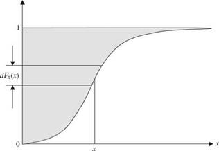
This expectation is also known as the mean of a random variable. It can be seen easily that the mean of a random variable is the first-order L-moment Л1. Geometrically, the mean or expectation of a random variable is the location of the centroid of the PDF or PMF. The second and third integrations in Eq. (2.30) indicate that the mean of a random variable is the shaded area shown in Fig. 2.11.

The following two operational properties of the expectation are useful:

1. The expectation of the sum of several random variables (regardless of their dependence) equals the sum of the expectation of the individual random

Fx(x) Figure 2.11 Geometric interpretation of the mean.

variable, that is,

( K K E akXk = ^2 akMk

k = і k = і

in which pk = E(Xk), for k = 1,2,…, K.

2. The expectation of multiplication of several independent random variables equals the product of the expectation of the individual random variables, that is,

E П Xk = П Mk (2.32)

k = 1 k = 1

Two other types of measures of central tendency of a random variable, namely, the median and mode, are sometimes used in practice. The median of a ran­dom variable is the value that splits the distribution into two equal halves. Mathematically, the median xmd of a continuous random variable satisfies

The median, therefore, is the 50th quantile (or percentile) of random variable X. In general, the 100pth quantile of a random variable X is a quantity xp that satisfies

P (X < xp) = Fx(xp) = p (2.34)

The mode is the value of a random variable at which the value of a PDF is peaked. The mode xmo of a random variable X can be obtained by solving the

following equation:

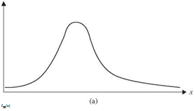
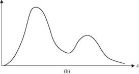
Referring to Fig. 2.12, a PDF could be unimodal with a single peak, bimodal with two peaks, or multimodal with multiple peaks. Generally, the mean, median, and mode of a random variable are different unless the PDF is symmetric and unimodal. Descriptors for the central tendency of a random variable are summarized in Table 2.1.

Example 2.10 (after Tung and Yen, 2005) Refer to Example 2.8, the pump reliability problem. Find the mean, mode, median, and 10 percent quantile for the random time to failure T.

Solution The mean of the time to failure, called the mean time to failure (MTTF), is the first-order moment about the origin, which is /xt —1250 h as calculated previ­ously in Example 2.8. From the shape of the PDF for the exponential distribution as shown in Fig. 2.7, one can immediately identify that the mode, representing the most likely time of pump failure, is at the beginning of pump operation, that is,

mo

Ш

Figure 2.12 Unimodal (a) and bimodal (b) distributions.

To determine the median time to failure of the pump, one can first derive the expression for the CDF from the given exponential PDF as

rt e-u/1250

Ft(t) = P(T < t) = ————— du = 1 — e-t/1250 for t > 0

к 1250 —

in which u is a dummy variable. Then the median time to failure tmd can be obtained, according to Eq. (2.33), by solving

Ft(tmd) = 1 — exp(-tmd/1250) = 0.5 which yields tmd = 866.43 h.

Similarly, the 10 percent quantile t0.1, namely, the elapsed time over which the pump would fail with a probability of 0.1, can be found in the same way as the median except that the value of the CDF is 0.1, that is,

Ft(t0.1) = 1 — exp(-0.1/1250) = 0.1 which yields t0.1 = 131.7 h.