Covariance and correlation coefficient
When a problem involves two dependent random variables, the degree of linear dependence between the two can be measured by the correlation coefficient pXyy, which is defined as
Corr(X, Y) = px, y = Cov(X, Y )laTay (2.47)
where Cov(X, Y) is the covariance between random variables X and Y, defined as
Cov(X, Y) = E[(X – ,ix)(Y – iiy)] = E(XY) – pPy (2.48)
Various types of correlation coefficients have been developed in statistics for measuring the degree of association between random variables. The one defined by Eq. (2.47) is called the Pearson product-moment correlation coefficient, or correlation coefficient for short in this and general use.
It can be shown easily that Cov(X^, X’2) = Corr(Xь X2), with X^ and X’2 being the standardized random variables. In probability and statistics, a random variable can be standardized as
X’ = (X – px)/ax (2.49)
Hence a standardized random variable has zero mean and unit variance. Standardization will not affect the skewness coefficient and kurtosis of a random variable because they are dimensionless.
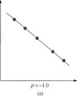
Figure 2.14 graphically illustrates several cases of the correlation coefficient. If the two random variables X and Y are statistically independent, then Corr(X, Y) = Cov(X, Y) = 0 (Fig. 2.14c). However, the reverse statement is not necessarily true, as shown in Fig. 2.14d. If the random variables involved are not statistically independent, Eq. (2.70) for computing the variance of the sum of several random variables can be generalized as
/ k K K-1 K
Var ]T akXk = ]T aal + 2 £ ]T akak, Cov(Xk, X„) (2.50)
k = 1 ) k = 1 k = 1 k=k+1
Example 2.12 (after Tung and Yen, 2005) Perhaps the assumption of independence of Pm, Im, and Em in Example 2.11 may not be reasonable in reality. One examines the historical data closely and finds that correlations exist among the three hydrologic random variables. Analysis of data reveals that Corr(Pm, Im) = 0.8, Corr(Pm, Em) = -0.4, and Corr(Im, Em) = – 0.3. Recalculate the standard deviation associated with the end-of-month storage volume.
|
|

 • •
• •
_ • • • . •
• • •
p = 0.8
(b)
|
|
||
|
|||
|
|||
|
|||
|
|||


Figure 2.14 Different cases of correlation between two random variables:
(a) perfectly linearly correlated in opposite directions; (b) strongly linearly correlated in a positive direction; (c) uncorrelated in linear fashion; (d) perfectly correlated in nonlinear fashion but uncorrelated linearly.
Solution By Eq. (2.50), the variance of the reservoir storage volume at the end of the month can be calculated as
Var(Sm+1) = ar (Pm) + Var(Im) + Var(Em) + 2 Cov(Pm, Im)
— 2 Cov(Pm, Em) — 2 Cov(Im, Em)
= Var(Pm) + Var(Im) + Var(Em) + 2 Corr(Pm, Im)o(Pm)o(Im)
— 2Corr(Pm, Em)&(Pm)&(Em) — 2 Corr(Im, Em)&(Im)&(Em) = (500)2 + (2000)2 + (1000)2 + 2(0.8)(500)(2000)
— 2(—0.4)(500)(1000) — 2(—0.3)(2000)(1000)
= 8.45(1000 m3)2
The corresponding standard deviation of the end-of-month storage volume is a(Sm+1) = V845 x 1000 = 2910 m3
In this case, consideration of correlation increases the standard deviation by 27 percent compared with the uncorrelated case in Example 2.11.
Example 2.13 Referring to Example 2.7, compute correlation coefficient between X and Y.
Solution Referring to Eqs. (2.47) and (2.48), computation of the correlation coefficient requires the determination of xx, xy, ax, and ay from the marginal PDFs of X and Y:
4 -t – 3×2 4 -t – 3 y2
fx(x) = ——— for 0 < x < 2 fy(y) = ——— for 0 < y < 2
as well as E(XY) from their joint PDF obtained earlier:

![]() 3( x2 + y2)
3( x2 + y2)
32
From the marginal PDFs, the first two moments of X and Y about the origin can be obtained easily as
Var(X) = E(X2) – (Mx)2 = 73/240 = Var(Y)
To calculate Cov(X, Y), one could first compute E(XY) from the joint PDF as
E(XY) = f ( xyfx, y(x, y) dxdy = |
J0 J0
Then the covariance of X and Y, according to Eq. (2.48), is Cov(X, Y) = E (XY) – nxny = -1/16 The correlation between X and Y can be obtained as


Leave a reply