Category Hydrosystems Engineering Reliability Assessment and Risk Analysis

Treatment of nonnormal stochastic variables

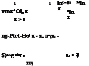
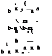
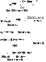
When nonnormal random variables are involved, it is advisable to transform them into equivalent normal variables. Rackwitz (1976) and Rackwitz and Fiessler (1978) proposed an approach that transforms a nonnormal distribu­tion into an equivalent normal distribution so that the probability content is preserved. That is, the value of the CDF of the transformed equivalent nor­mal distribution is the same as that of the original nonnormal distribution at the design point x*. Later, Ditlvesen (1981) provided the theoretical proof of the convergence property of the normal transformation in the reliability algo­rithms searching for the design point. Table 4.3 presents the normal equivalent for some nonnormal distributions commonly used in reliability analysis.

By the Rackwitz (1976) approach, the normal transform at the design point x* satisfies the following condition:

Fk (xk-) = ф(Xk – ‘k-N ) = Ф(гІ) for k = 1,2,…, K (4.59)

V ak*N J

in which Fk (xk-) is the marginal CDF of the stochastic basic variable Xk having values at xk-, ‘k-N and ok-N are the mean and standard deviationas of the normal equivalent for the kth stochastic basic variable at Xk = xk-, and zk – = Ф-1[Fk(xk-)] is the standard normal quantile. Equation (4.59) indicates that the marginal probability content in both the original and normal transformed spaces must be preserved. From Eq. (4.59), the following equation is obtained:

‘k-N = xk – – Zk-Ok-N (4.60)

Note that ‘k-N and ok-N are functions of the expansion point x-. To obtain the standard deviation in the equivalent normal space, one can take the derivative on both sides of Eq. (4.59) with respect to xk, resulting in

Treatment of nonnormal stochastic variablesfk(xk-) = – Xф (xLz»2L

Ok-N Ok-N

Подпись: Ok-N Подпись: Ф (Zk-) f k (xk-) Подпись: (4.61)

in which fk ( ) and ф ( ) are the marginal PDFs of the stochastic basic variable Xk and the standard normal variable Zk, respectively. From this equation, the normal equivalent standard deviation ok-N can be computed as

Therefore, according to Eqs. (4.60) and (4.61), the mean and standard deviation of the normal equivalent of the stochastic basic variable Xk can be calculated.

It should be noted that the normal transformation uses only the marginal distributions of the stochastic basic variables without regarding their correla­tions. Therefore, it is, in theory, suitable for problems involving independent

Distribution
of X


Equivalent standard normal variable
ZN = Ф-1[Рх (x„)]


PDF, fx(xt)


ON


ln(xt) Mln x

Oln x


Treatment of nonnormal stochastic variables

2


Lognormal


xt Oln x


Treatment of nonnormal stochastic variables

Exponential


Treatment of nonnormal stochastic variables

– -2- + P(xt – xo)


Ф (Zt)

fx ( xt)

Ф (Zt)

fx ( xt)


Gamma


x – $ ( x – $

– exp


Treatment of nonnormal stochastic variables

Type 1

extremal

(max)


Ф 1 < exp


– exp –


в


—oo < x < oo


Treatment of nonnormal stochastic variables

axm


1


axm


Ф (Zt)

fx ( xt)


Triangular


mxb


1


mxb


1 / xt – a b — a


(b – a)ф(Zt)


Uniform


NOTE: In all cases, mn = xt – ZtON. SOURCE: After Yen et al. (1986).


Подпись: 181

nonnormal random variables. When stochastic basic variables are nonnormal but correlated, additional considerations must be given in the normal transfor­mation (see Sec. 4.5.7).

To incorporate the normal transformation for nonnormal uncorrelated stochastic basic variables, the Hasofer-Lind AFOSM algorithm for problems having uncorrelated nonnormal stochastic variables involves the following steps:

Step 1: Select an initial trial solution x(r).

Step 2: Compute the mean and standard deviation of the normal equivalent

using Eqs. (4.60) and (4.61) for those nonnormal stochastic basic variables.

For normal stochastic basic variables, pkN,(r) = дk and akN,(r) = ak.

Step 3: Compute W(x(r>) and the corresponding sensitivity coefficient vector

sx,(r) •

Step 4: Revise solution point x(r+i> according to Eq. (4.52) with the mean

and standard deviations of nonnormal stochastic basic variables replaced by

Treatment of nonnormal stochastic variables Подпись: "MN ,(r )У sx,(r) W (x (r)) Sx,(r) D N ,(r) Sx,(r) Подпись: (4.62)

their normal equivalents, that is,

Step 5: Check if x(r) and x(r+1) are sufficiently close. If yes, compute the reli­ability index ^AFOSM according to Eq. (4.47) and the corresponding reliability ps = Ф)^^); then, go to step 5. Otherwise, update the solution point by letting x(r) = x(r+1) and return to step 2.

Step 6: Compute the sensitivity of the reliability index and reliability with respect to changes in stochastic basic variables according to Eqs. (4.48), (4.49), and (4.50) with Dx replaced by DxN at the design point x*.

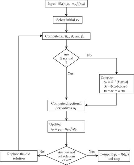
As for the Ang-Tang AFOSM algorithm, the iterative algorithms described previously can be modified as follows (also see Fig. 4.10):

Step 1: Select an initial point x(r) in the parameter space.

Step 2: Compute the mean and standard deviation of the normal equivalent using Eqs. (4.60) and (4.61) for those nonnormal stochastic basic variables. For normal stochastic basic variables, pkN,(r) = Pk and akN,(r) = &k.

Step 3: At the selected point x(r), compute the mean and variance of the performance function W(x(r>) according to Eqs. (4.56) and (4.44), respect­ively.

Step 4: Compute the corresponding reliability index в(г) according to Eq. (4.8).

Step 5: Compute the values of the normal equivalent directional derivative akN,(r), for all k = 1,2, •••, K, according to Eq. (4.46), in that the standard

deviations of nonnormal stochastic basic variables ak’s are replaced by the corresponding OkN,(r)’s.

Step 6: Using во) and akN,(r) obtained from steps 3 and 5, revise the location of expansion point xо+1) according to

Подпись: (4.63)Xk,(r + 1) = PkN,(r) – akN,(r)во)akN,(r) k = 1, 2, … , K

Step 7: Check if the revised expansion point x(r+p differs significantly from the previous trial expansion point x(r). If yes, use the revised expansion point as the new trial point by letting xо) = xо+p, and go to step 2 for an­other iteration. Otherwise, the iteration is considered complete, and the latest reliability index во) is used to compute the reliability ps = Ф(во)).

Step 8: Compute the sensitivity of the reliability index and reliability with respect to changes in stochastic basic variables according to Eqs. (4.47), (4.48), and (4.49) with D x replaced by DxN at the design point x*.

Example 4.10 (Independent, nonnormal) Refer to the data in Example 4.9 for the

storm sewer reliability analysis problem. Assume that all three stochastic basic vari­ables are independent random variables having different distributions. Manning’s roughness n has a normal distribution; pipe diameter D, lognormal; and pipe slope S, Gumbel distribution. Compute the reliability that the sewer can convey an inflow discharge of 35 ft3/s by the Hasofer-Lind algorithm.

Solution The initial solution is taken to be the means of the three stochastic basic vari­ables, namely, xq) = p, x = (pn, xd, xs) = (0.015, 3.0, 0.005)г. Since the stochastic basic variables are not all normally distributed, the Rackwitz normal transformation is applied. For Manning’s roughness, no transformation is required because it is a normal stochastic basic variable. Therefore, fin, N,(1) = Xn = 0.015 and an, n,(i) = an = 0.00075.

For pipe diameter, which is a lognormal random variable, the variance and the mean of log-transformed pipe diameter can be computed, according to Eqs. (2.67a) and (2.67b), as

Подпись: .2 'ln D

Treatment of nonnormal stochastic variables

= ln( 1 + 0.022) = 0.0003999

The standard normal variate zd corresponding to D = 3.0 ft. is

zd = [ln( 3) — xln D iMn D = 0.009999

Then, according to Eqs. (4.60) and (4.61), the standard deviation and the mean of normal equivalent at D = 3.0 ft. are, respectively,

Xd, N,(1) = 2.999 ад, n,(1) = 0.05999

For pipe slope, the two parameters in the Gumbel distribution, according to Eqs. (2.86a) and (2.86b), can be computed as

в = ,°S = 0.0001949

V1.645

§ = дS — 0.577в = 0.004888

The value of reduced variate Y = (S — §)/в at S = 0.005 is Y = 0.577, and the corresponding value of CDF by Eq. (2.85a) is Fev1(Y = 0.577) = 0.5703. According to Eq. (4.59), the standard normal quantile corresponding to the CDF of 0.5703 is Z = 0.1772. Based on the available information, the values of PDFs for the standard normal and Gumbel variables, at S = 0.005, can be computed as ф(Z = 0.1722) = 0.3927 and /"ev/Y = 0.577) = 1643. Then, by Eqs. (4.61) and (4.60), the nor­mal equivalent standard deviation and the mean for the pipe slope, at S = 0.005, are

Hs n (1) = 0.004958 &s n (1) = 0.000239

At x(1) = (0.015, 3.0, 0.005/, the normal equivalent mean vector for the three stochas­tic basic variables is

VN ,(1) = (Дп, N ДЬ VD, N ДЬ д-S, N,(1)/ = (°.°15, 2.999, °.°04958)< and the covariance matrix is

2

an, N

0

0

0.000752

0

0

D N,(1) =

1

О О

2

aD, N 0

0

2

aS, N.

=

1

О О

0.05992

0

0

0.0002392 _

At x(1), the sensitivity vector sx,(1) is

sX;(1) = (9W/дn, dW/дD, dW/дS) = (—2734, 36.50, 4101/

and the value of the performance function W(n, D, S) = 6.010, is not equal to zero. This implies that the solution point x(1) does not lie on the limit-state surface. Apply­ing Eq. (4.62) using normal equivalent means vn and variances Dxn and the new solution x(2) can be obtained as x(2) = (0.01590, 2.923, 0.004821/. Then one checks the difference between the two consecutive solutions as

9 = | x(1) — x(2)| = [(0.0159 — 0.015)2 + (2.923 — 3.0)2 + (0.004821 — 0.005)2]a5 = 0.07729

which is considered large, and therefore, the iteration continues. The following table lists the solution point x(r), its corresponding sensitivity vector sx,(r), and the vector of directional derivatives aN,(r) in each iteration. The iteration stops when the dif­ference between the two consecutive solutions is less than 0.001 and the value of the performance function is less than 0.001.

Iteration

Var.

x(r)

,(r)

&N,(r)

sx,(r)

aN,(r)

x (r +1)

r

= 1

n

0.1500 x

10—01

0.1500 x 10—01

0.7500 x 10—03

—0.2734 x 10+04

—0.6497 x 10+00

0.1590

x 10—01

D

0.3000 x

10+01

0.2999 x 10+01

0.5999 x 10—01

0.3650 x 10+02

0.6938 x 10+00

0.2923

x 10+01

S

о

Ql

о

о

о

X

10—02

0.4958 x 10—02

0.2390 x 10—03

0.4101 x 10+04

0.3106 x 10+00

0.4821

x 10—02

5

= 0.7857 x 10—01

W = 0.6010 x 10+01

в = 0.0000 x 10+00

r

= 2

n

0.1590 x

10—01

0.1500 x 10—01

0.7500 x 10—03

—0.2229e+04

—0.6410e+°°

0.1598

x 10—01

D

0.2923 x

10+01

0.2998 x 10+01

0.5845 x 10—01

0.3237 x 10+02

0.7255 x 10+00

0.2912

x 10+01

S

0.4821 x

10—02

0.4944 x 10—02

0.1778 x 10—03

0.3675 x 10+04

0.2505 x 10+00

0.4853

x 10—02

5

= 0.1113 x 10—01

W = 0.4371 x 10+00

в = 0.1894 x 10+01

r

= 3

n

0.1598 x

10—01

0.1500 x 10—01

0.7500 x 10—03

—0.2190 x 10+04

—0.6369 x 10+00

0.1598

x 10—01

D

0.2912e+01

0.2998e+01

0.5823 x 10—01

0.3210 x 10+02

0.7247 x 10+00

0.2912

x 10+01

S

0.4853 x

10—02

0.4950 x 10—02

0.1880 x 10—03

0.3607 x 10+04

0.2630e+00

0.4849

x 10—02

5

= 0.1942 x 10—04

W = 0.2147 x 10—02

в = 0.2049 x 10+01

r

= 4

n

0.1598 x

10—01

0.1500 x 10—01

0.7500 x 10—03

—0.2190 x 10+04

—0.6373 x 10+01

0.1598

x 10—01

D

0.2912 x

10+01

0.2998 x 10+01

0.5823 x 10—01

0.3210 x 10+02

0.7249 x 10+00

0.2912

x 10+01

S

0.4849 x

10—02

0.4949 x 10—02

0.1867 x 10—03

0.3609 x 10+04

0.2614 x 10+00

0.4849

x 10—02

5

= 0.2553 x 10—04

W = 0.3894 x 10—05

в = 0.2050 x 10+01

After four iterations, the solution converges to the design point x* = (n*, D*, S*)г = (0.01598, 2.912, 0.004849)г. At the design point x*, the mean and standard deviation of the performance function W can be estimated by Eqs. (4.42) and (4.43), respectively, as

Hw* = 5.285 and aw* = 2.578

The reliability index then can be computed as в* = iw l°w* = 2.050, and the corre­sponding reliability and failure probability can be computed, respectively, as

ps = Ф(в*) = 0.9798 pf = 1 — ps = 0.02019

Finally, at the design point x*, the sensitive of the reliability index and reliability with respect to each of the three stochastic basic variables can be computed by Eqs. (4.49) and (4.50). The results are shown in columns (4) to (7) in the following table:

Variable

(1)

x

(2)

aN,* (3)

дв/д z (4)

д ps |д z (5)

дв/д x (6)

дps/д x (7)

хдв/вдx (8)

xд psl psд x (9)

n

0.01594

—0.6372

0.6372

0.03110

849.60

41.46

6.623

0.6762

D

2.912

0.7249

—0.7249

—0.03538

—12.45

—0.61

—17.680

—1.8060

S

0.00483

0.2617

—0.2617

—0.01277

—1400.00

— 68.32

—3.312

—0.3381

The sensitivity analysis yields a similar indication about the relative importance of the stochastic basic variables, as in Example 4.9.

Algorithms of AFOSM for independent normal parameters

Подпись: W '(z (r)) a |Vz' W'(Z (r ))| (r>

Подпись: Z (r +1) ( a(r ) z (r )) a(r )
Подпись: for r = 1,2,... (4.51)

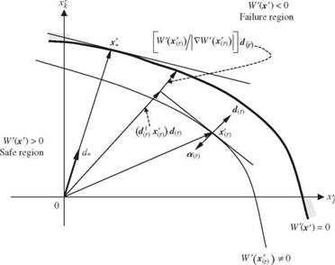
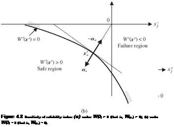
Hasofer-Lind algorithm. In the case that X are independent normal stochastic basic variables, standardization of X according to Eq. (4.30) reduces them to independent standard normal random variables Z’ with mean 0 and covariance matrix I, with I being a K x K identity matrix. Referring to Fig. 4.8, based on the geometric characteristics at the design point on the failure surface, Hasofer and Lind (1974) proposed the following recursive equation for determining the design point z (.

Подпись:Подпись: for r = 1,2, 3,... (4.52)

Подпись: Vx ) S(r) — W (x (r)) s(r)D xs (r)
Подпись: x (r + 1) — + D xs(r)

in which subscripts (r) and (r + 1) represent the iteration numbers, and —a denotes the unit gradient vector on the failure surface pointing to the failure region. Referring to Fig. 4.9, the first terms of Eq. (4.51), — (—al(r z(r))a(r), is a projection vector of the old solution vector z (r) onto the vector —a (r) emanating from the origin. The quantity W'(z(r))/|VW'(z(r))| is the step size to move from W'(z(r)) to W'(z’) = 0 along the direction defined by the vector —a(r). The second term is a correction that further adjusts the revised solution closer to the limit-state surface. It would be more convenient to rewrite the preceding recursive equation in the original лт-space as

Based on Eq. (4.52), the Hasofer-Lind AFOSM reliability analysis algorithm for problems involving uncorrelated, normal stochastic variables the can be outlined as follows:

Step 1: Select an initial trial solution x(r).

Step 2: Compute W(x(r>) and the corresponding sensitivity coefficient vector

s (r).

Step 3: Revise solution point x(r+1), according to Eq. (4.52).

Step 4: Check if x(r) and x(r+1) are sufficiently close. If yes, compute the reli­ability index eAFOSM according to Eq. (4.47) and the corresponding reliability

Algorithms of AFOSM for independent normal parameters

Algorithms of AFOSM for independent normal parameters

Figure 4.9 Geometric interpretation of Hasofer-Lind algorithm in standard­ized space.


ps = ФС^їге^; then, go to step 5. Otherwise, update the solution point by letting x(r) = x(r+1> and return to step 2.

Step 5: Compute the sensitivity of the reliability index and reliability with respect to changes in stochastic basic variables according to Eqs. (4.48), (4.49), and (4.50).

It is possible that a given performance function might have several design points. In the case that there are J such design points, the reliability can be calculated as

Ps = №(^afosm)]J (4.53)

Ang-Tang algorithm. The core of the updating procedure of Ang and Tang (1984) relies on the fact that according to Eq. (4.47), the following relationship should be satisfied:

K

У> (pk – Xk> – ak>P*vk) = 0 (4.54)

k=1

Since the variables X are random and uncorrelated, Eq. (4.35) defines the fail­ure point within the first-order context. Hence Eq. (4.47) can be decomposed into

Подпись: (4.55)Xk = Pk – ak>в*°k for k = 1, 2,…, K

Ang and Tang (1984) present the following iterative procedure to locate the de­sign point x+ and the corresponding reliability index ^AFOSM under the condition that stochastic basic variables are independent normal random variables. The Ang-Tang AFOSM reliability algorithm for problems involving uncorrelated normal stochastic variables has the following steps (Fig. 4.10):

Step 1: Select an initial point x(r) in the parameter space. For practicality, the point iix where the means of stochastic basic variables are located is a viable starting point.

Algorithms of AFOSM for independent normal parameters

Figure 4.10 Flowchart of the Ang-Tang AFOSM reliability analysis involving uncorre­lated variables.

Step 2: At the selected point x (r), compute the mean of the performance func­tion W (X) by

MW = w(x(r)) + s r)(^x – x(r)) (4.56)

and the variance according to Eq. (4.44).

Step 3: Compute the corresponding reliability index ) according to Eq. (4.34).

Step 4: Compute the values of directional derivative ak for all k = 1, 2,, K according to Eq. (4.46).

Step 5: Revise the location of expansion point x(r+p according to Eq. (4.56) using ak and в(г) obtained from steps 3 and 4.

Step 6: Check if the revised expansion point x(r +p differs significantly from the previous trial expansion point x (r). If yes, use the revised expansion point as the new trial point by letting x(r) = x(r+p, and go to step 2 for an additional iteration. Otherwise, the iteration procedure is considered complete, and the latest reliability index is eAFOSM and is to be used in Eq. (4.10) to compute the reliability ps.

Step 7: Compute the sensitivity of the reliability index and reliability with respect to changes in stochastic basic variables according to Eqs. (4.48), (4.49), and (4.50).

Referring to Eq. (4.8), the reliability is a monotonically increasing function of the reliability index в, which, in turn, is a function of the unknown failure point. The task to determine the critical failure point x+ that minimizes the reliability is equivalent to minimizing the value of the reliability index в. Low and Tang (1997), based on Eqs. (4.31a) and (4.31b) developed an optimization procedure in Excel by solving

Mm в = ^J(x – fxxУC-1(x – fxx) 57)

subject to W(x) = 0

Owing to the nature of nonlinear optimization, both AFOSM-HL and AFOSM – AT algorithms do not necessarily converge to the true design point associated with the minimum reliability index. Madsen et al. (1986) suggested that dif­ferent initial trial points be used and that the smallest reliability index be cho­sen to compute the reliability. To improve the convergence of the Hasofer-Lind algorithm, Liu and Der Kiureghian (1991) proposed a modified objective func­tion for Eq. (4.31a) using a nonnegative merit function.

Example 4.9 (Uncorrelated, normal) Refer to Example 4.5 for a storm sewer relia­bility analysis problem with the following data:

Variable

Mean

Coefficient of variation

n (ft1/6)

0.015

0.05

D (ft)

3.0

0.02

S (ft/ft)

0.005

0.05

Assume that all three stochastic basic variables are independent normal random variables. Compute the reliability that the sewer can convey an inflow discharge of 35 ft3/s using the AFOSM-HL algorithm.

Solution The initial solution is taken to be the means of the three stochastic basic variables, namely, x(1) = fix = (^n, xd, xs)t = (0.015, 3.0, 0.005^. The covariance matrix for the three stochastic basic variables is

0

0

0.000752

0

0

D x =

0

0

D

0

0

aS.

=

0

0

0.062

0

0

0.000252

For this example, the performance function Qc — Ql is

W(n, D, S) = Qc — Ql = 0.463n—1D8/3S1/2 — 35

Note that because the W(^n, гD, XS) = 6.010 > 0, the mean point fix is located in the safe region. At x(1) = fix, the value of the performance function W(n, D, S) = 6.010, which is not equal to zero. This implies that the solution point x(1), does not lie on the limit-state surface. By Eq. (4.52), the new solution x(2) can be obtained as x(2) = (0.01592,2.921,0.004847). Then one checks the difference between the two consecutive solution points as

5 = |x (1) — x (2)| = [(0.01592 — 0.015)2 + (2.921 — 3.0)2 + (0.004847 — 0.005)2]05 = 0.07857

which is considered large, and therefore, the iteration continues. The following table lists the solution point x(r), its corresponding sensitivity vector s(r), and the vector of directional derivatives a (r) in each iteration. The iteration stops when the differ­ence between the two consecutive solutions is less than 0.001 and the value of the performance function is less than 0.001.

Iteration

Var.

x (r )

s (r )

a(r)

x(r+1)

r = 1

n

0.1500 x 10—01

—0.2734 x 10+04

—0.6468 x 10+00

0.1592 x 10—01

D

0.3000 x 10—01

0.3650 x 10+02

0.6907 x 10+00

0.2921 x 10+01

S

0.5000 x 10—02

0.4101 x 10+04

0.3234 x 10+00

0.4847 x 10—02

5 = 0.7857 x 10—01

W = 0.6010 x 10+01

в =

0.0000 x 10+00

r = 2

n

0.1592 x 10—01

—0.2226 x 10+04

—0.6138 x 10+00

0.1595 x 10—01

D

0.2921 x 10+01

0.3239 x 10+02

0.7144 x 10+00

0.2912 x 10+01

S

0.4847 x 10—02

0.3656 x 10+04

0.3360 x 10+00

0.4827 x 10—02

5 = 0.9584 x 10—02

W = 0.4421 x 10+00

в =

0.1896 x 10+01

(Continued)

Iteration

Var.

x (r )

s (r )

a(r)

x(r+1)

r = 3

n

0.1595 x 10—01

—0.2195 x 10+04

—0.6118 x 10+00

0.1594 x 10—01

D

0.2912 x 10—01

0.3209 x 10+02

0.7157 x 10+00

0.2912 x 10+01

S

0.4827 x 10—02

0.3625 x 10+04

0.3369 x 10+00

0.4827 x 10—02

S = 0.1919 x 10—03

W = 0.2151 x 10—02

в

= 0.2056 x 10+01

r = 4

n

0.1594 x 10—01

—0.2195 x 10+04

—0.6119 x 10+00

0.1594 x 10—01

D

0.2912 x 10+01

0.3210 x 10+02

0.7157 x 10+00

0.2912 x 10+01

S

0.4827 x 10—02

0.3626 x 10+04

0.3369 x 10+00

0.4827 x 10—02

S = 0.3721 x 10—05

W = 0.2544 x 10—06

в

= 0.2057 x 10+01

After four iterations, the solution converges to the design point x* = (n*, D*, S*)г = (0.01594, 2.912, 0.004827)г. At the design point x*, the mean and standard deviation ofthe performance function W canbe estimated, by Eqs. (4.42) and (4.43), respectively, as

pw* = 5.536 and aw* = 2.691

The reliability index then can be computed as в* = IW/&w* = 2.057, and the corre­sponding reliability and failure probability can be computed, respectively, as

ps = Ф(в*) = 0.9802 pf = 1 — ps = 0.01983

Finally, at the design point x*, the sensitivity of the reliability index and reliabil­ity with respect to each of the three stochastic basic variables can be computed by Eqs. (4.49) and (4.50). The results are shown in columns (4) to (7) ofthe following table:

Variable

(1)

x*

(2)

a*

(3)

9в/9 X (4)

9ps/9 X (5)

9в/9 x (6)

9 ps/9 x (7)

хдв/в’д X (8)

хдps/ps 9x (9)

n

0.01594

— 0.6119

0.6119

0.02942

815.8

39.22

6.323

0.638

D

2.912

0.7157

—0.7157

—0.03441

—11.9

—0.57

—16.890

—1.703

S

0.00483

0.3369

— 0.3369

— 0.01619

—1347.0

—64.78

—3.161

—0.319

From the preceding table, the quantities 9в/9х’к and 9ps/9x’k show the sensitivity of the reliability index and reliability for one standard deviation change in the k-th stochastic basic variable, whereas 9в/9Xk and 9ps/9Xk correspond to one unit change of the k-th stochastic basic variables in the original space. As can be seen, the sensitivity of в and ps associated with Manning’s roughness coefficient is positive, whereas those for pipe size and slope are negative. This indicates that an increase in Manning’s roughness coefficient would result in an increase in в and ps, whereas an increase in slope and/or pipe size would decrease в and ps. The indication is confusing from a physical viewpoint because an increase in Manning’s roughness coefficient would decrease the flow-carrying capacity of the sewer, whereas, on the other hand, an increase in pipe diameter and/or pipe slope would increase the sewer’s conveyance capacity. The problem is that the sensitivity coefficients for в and ps are taken relative to the design point on the failure surface; i. e., a larger Manning’s would be farther from the system’s mean condition, thus resulting in a larger value of в. However, larger values ofpipe diameter or slope would be closer to the system’s mean condition, thus resulting in a smaller value of в. Thus the sign of the sensitivity coefficients is deceiving, but their magnitude is useful, as described in the following paragraphs.

Furthermore, one can judge the relative importance of each stochastic basic vari­able based on the absolute values of the sensitivity coefficients. It is generally difficult to draw a meaningful conclusion based on the relative magnitude of дв/дx and дps/dx because units of different stochastic basic variables are not the same. Therefore, sensi­tivity measures not affected by the dimension of the stochastic basic variables, such as дв/дx’ and дps/дx’, generally are more useful. With regard to a one standard deviation change, for example, pipe diameter is significantly more important than pipe slope.

Algorithms of AFOSM for independent normal parameters

An alternative sensitivity measure, called the relative sensitivity or the partial elasticity (Breitung, 1993), is defined as

Failure point)

In cases for which several stochastic basic variables are involved in a perfor­mance function, the number of possible combinations of such variables satis­fying W (x) = 0 is infinite. From the design viewpoint, one is more concerned with the combination of stochastic basic variables that would yield the lowest reliability or highest failure probability. The point on the failure surface asso­ciated with the lowest reliability is the one having the shortest distance to the point where the means of the stochastic basic variables are located. This point is called the design point (Hasofer and Lind, 1974) or the most probable failure point (Shinozuka, 1983).

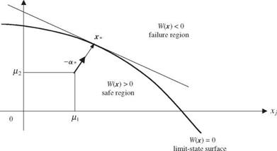
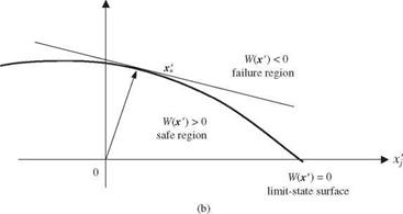
Consider that X = (X1,X2,…,XK)t are K uncorrelated stochastic basic variables having a vector mean px and covariance matrix Dx. The original stochastic basic variables X can be standardized into X’ according to Eq. (4.30). The standardization procedure maps the failure surface in the original x-space onto the corresponding failure surface in x’-space, as shown in Fig. 4.6. Hence the design point in x ‘-space is the one that has the shortest distance from the

Xk

Failure point)

(a)


x’

Failure point)

Figure 4.6 Performance function in the original and standardized spaces: (a) original space; (b) standardized space.


Подпись: Minimize subject to Failure point) Подпись: ^ x'l k=1 Подпись: (4.31a) (4.31b)

failure surface W'(x 0 = 0 to the origin x’ = 0. Such a point can be found by solving

This constrained nonlinear minimization problem can be converted into an unconstrained minimization problem using the Lagrangian function:

Подпись: (4.32)Minimize L(x’, %) = (x’tx 7)1/2 + f W'(x’)

Failure point) Failure point) Failure point) Подпись: x7 -^ + f*Vx W'(x *) = 0 |x *| W 7(x *) = 0 Подпись: (4.33a) (4.33b)

in which f is the Lagrangian multiplier, which is unrestricted in sign. The solution to Eq. (4.32) can be obtained by solving the following two equations simultaneously, that is,

Подпись: (4.34)in which Vx = (д/д x1, d/dx2,…, d/dxK )t is a gradient operator. FromEq. (4.33a), the design point x * can be expressed as

x * = f * |x *|Vx7 W ‘(x *)

Furthermore, from Eq. (4.34), the distance between the origin x’ = 0 and the design point x * can be obtained as

|x *| = If* ||x *|[VX 7 W ‘(x * )Vx W'(x *)]1/2 = If* ||x *||Vx7 W ‘(x *)| (4.35)

from which the value of the optimal Lagrangian multiplier x* can be determined as

f* = sign[W 7(0)]|Vx W 7( x* )|-1 (4.36)

Substituting Eq. (4.36) into Eq. (4.34) determines the location of the design point as

V W'(x 7)

x* = – sign[W'(O)]|x*| rox * = – sign[W'(0)]|x*|a* (4.37)

|Vx7 W (x *)

Подпись: |x 'J = -sign[W '(0)]atx ( = -sign[W '(0)]- Failure point) Подпись: (4.38)

in which a* = Vx W 7(x *)/|Vx – W 7(x **)| is a unit vector emanating from the design point x’* and pointing toward the safe region. Referring to Fig. 4.6, where the mean point fux is located in the safe region, hence W'(0) > 0 [or W(px) > 0], and the corresponding – sign[W'(0)]a* is a unit vector emanating from the origin x7 = 0 and pointing to the design point x*. The elements of a* are called the directional derivatives representing the value of the cosine angle between the gradient vector Vx W'(x **) and axes of the standardized variables. Geometri­cally, Eq. (4.37) shows that the vector, x** is perpendicular to the tangent hyper­plane passing through the design point. The shortest distance can be expressed as

Подпись: (4.39a)Recall that Xk = fik + akX’k, for k = 1, 2,, K. By the chain rule in calculus,

d W'(Xr) d w (X) dXk d w (X)

d Xk ~ d Xk Щ ~ d Xk ak

or in matrix form as

Vx W'(X’) = D^VxW (X) (4.39b)

Подпись: |x * Failure point) Подпись: (4.40)

Then Eq. (4.38) can be written, in terms of the original stochastic basic variables X, as

in which x* = (x1+, x2*,…, xK* )* is the point in the original variable x-space that can be easily determined from the design point x * in x’-space as x* = fix + D У2x *. It will be shown in the next subsection that the shortest distance from the origin to the design point |x *|, in fact, is the absolute value of the reliabil­ity index based on the first-order Taylor series expansion of the performance function W (X) with the expansion point at x*.

Example 4.8 (Linear performance function) Consider that the failure surface is a hyperplane given by

K

W (X) = a + £) akXk

k=1

or in vector form as W(X) = Oq + a* X = 0, with a’s being the coefficients and X being the random variables. Assume that X are uncorrelated random variables with the mean vector fix and covariance matrix Dx. It can be shown that the MFOSM reliability index computed by Eq. (4.29) with /iw = a0 + a* fix and aW = a* Dxa is the AFOSM reliability index.

To show that the original random variables X are first standardized by Eq. (4.30), therefore, in terms of the standardized random variables X’, the preceding linear failure surface can be expressed as

W'(X’) = b0 + b* X’ = 0

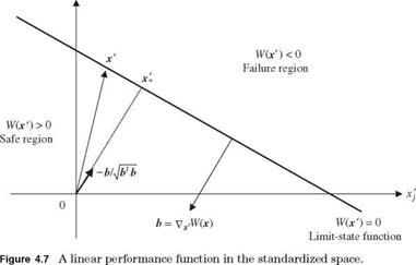
in which bo = Oq + a*fix and b* = a*DУ2. In Fig. 4.7, let the lower half space con­taining the origin of x ‘-space be designated as the safe region. This would require

bj = Oq + a*fix > 0.

Referring to Fig. 4.7, the gradient of W'(X’) is b, which is a vector perpendicular to the failure hyperplane defined by W'(X’) = 0 pointing in the direction of the safe set. Therefore, the vector —a = —bjlb*b is a unit vector emanating from x’ = 0 toward the failure region, as shown in Fig. 4.7. For any vector x’ landing on the

xk

Failure point)

failure hyperplane defined by W'(x’) = 0, the following relationship holds:

—2bl x’ 60

/ЪЪ = TPb

Note that the left-hand side is the length of the vector x’ projected on the unit vec­tor —Ы4¥Ъ, which is the shortest distance from x’ = 0 to the failure hyperplane. Therefore, b0/Vb1 b is the reliability index, that is,

e = 60 = ap + a

ЪЪ л/a Dx a aw

As shown, when the performance function is linear involving uncorrelated stochastic basic variables, the reliability index is the ratio of the expected value of the perfor­mance function to its standard deviation. Furthermore, the MFOSM method would yield the same results as the AFOSM method.

4.1.2 First-order approximation of performance function at the design point

Referring to Eqs. (4.20) and (4.21), the first-order approximation of the perfor­mance function W (X), taking the expansion point xo = x*, is

K

W(X) sk*(Xk — xk*) = s*(X — x*) (4.41)

k=i

in which s* = (sn, s2*,, sK*), a vector of sensitivity coefficients of the per­formance function W (X) evaluated at the expansion point x* that lies on the
limit-state surface, that is,

Подпись:Подпись: Sk* =for k = 1,2,…, K

X=x*

note that W(x*) is not on the right-hand-side of Eq. (4.41) because W(x*) = 0. Hence, at the expansion point x*, the expected value and the variance of the performance function W(X) can be approximated according to Eqs. (4.24) and (4.25) as

f^w ^ s *(Mx x*) (4.42)

al « s CXs* (4.43)

in which fj, x and Cx are the mean vector and covariance matrix of the stochastic basic variables, respectively. If the stochastic basic variables are uncorrelated, Eq. (4.43) reduces to

K

Подпись: (4.44)2 _ c.2 „2

aw = Sk*ak

k = 1

in which ak is the standard deviation of the kth stochastic basic variable Xk.

Since a* = s*/|s*|, when stochastic basic variables are uncorrelated, the standard deviation of the performance function W (X) alternatively can be ex­pressed in terms of the directional derivatives as

K

aw = ^2 ak*Sk*ak (4.45)

k=1

where ak* is the directional derivative for the kth stochastic basic variable at the expansion point x*

Sk ak

Failure point)


for k = 1, 2,…, K


(4.46a)


or, in matrix form,

Подпись: (4.46b)D 1/2Vx W (x*)

| D 1/2Vx W (x*)|

which is identical to the one defined in Eq. (4.37) according to Eq. (4.39). With the mean and standard deviation of the performance function W (X) computed

at x*, the AFOSM reliability index ^afosm given in Eq. (4.34) can be determined as

вafosm = ^ = ^k=1KSk*(lXk – Xk*} (4.47)

Z_jk = 1 ak*sk*Gk

The reliability index eAFOSM also is called the Hasofer-Lind reliability index.

Once the value of eAFOSM is computed, the reliability can be estimated by Eq. (4. 10) as Ps = $^afosm). Since eAFOSM = sign[W40)]|x*|, the sensitiv­ity of eAFOSM with respect to the uncorrelated, standardized stochastic basic variables is

x’

Vx’ eAFOSM = sign[W/(0)]Vx’|x(| = sign[W 40)]—^ = – a* (4.48)

|x *

Note that Vx в is a vector showing the direction along which the rate change in the value of the reliability index в increases most rapidly. This direction is indicated by – a* regardless whether the position of the mean of the stochastic basic variables fxx is in the safe region W40) > 0 or failure zone W40) < 0. As shown in Fig. 4.8, the vector – a* points to the failure region, and moving along – a* would result in a more negative-valued W'(x0. This is, geometri­cally, equivalent to pushing the limit-state surface W'(x’) = 0 further away from x’ = 0 in Fig. 4.8a and closer to x’ = 0 in Fig. 4.8b. Hence, moving along the direction of – a* at the design point x* would make the value of the relia­bility index в more positive under W40) > 0, whereas the value of в would be less negative under W40) < 0.

In both cases, the value of the reliability index increases along – a*. Alge­braically, as one moves along – a*, the current value of the limit-state surface W'(x’) changes from 0 to a negative value, that is, W'(x’) = – c, for c > 0. This implies a new limit state for the system defined by W'(x’) = R(x’) – L(x’) + c = 0. The introduction of a positive-valued c in the performance function could mean an increase in resistance, that is, W'(x’) = [R(x0 + c] – L(x’) = 0, or a decrease in load, that is, W'(x’) = R(x’) – [L(x’) – c] = 0. In either case, the reliability index and the corresponding reliability for the system would increase along the direction of – a*.

Подпись: ak* Подпись: ^AFOSM 4 ~щ~) Подпись: ЭвAFOSM d Xk Подпись: Gk Подпись: for k = 1, 2,..., K (4.49a)

Equation (4.48) indicates that moving along the direction of a* at the design point x*, the values of the reliability index would decrease and that – ak* is the rate of change in вАго:зМ owing to a one standard deviation change in stochastic basic variable Xk at X = x*. Therefore, the relationship between Vx в and Vxв can be expressed as

or, in matrix form, as

Failure point)

It also can be shown easily that the sensitivity of reliability or failure probability with respect to each stochastic basic variable along the direction of a* can be computed as

Failure point)

Failure point)

ak*ф (eAFOSM)

ak* Ф (^afosm)

®k


(4.50a)


or in matrix form as

Подпись:Vx; Ps = —Ф (eAFOSM)a*

Vx, Ps = Ф (^afosm)Vx, ^afosm = —Ф (^afosm) D x1/2 a*

These sensitivity coefficients would reveal the relative importance of each stochastic basic variable for their effects on reliability or failure probability.

Advanced First-Order Second-Moment (AFOSM) Method

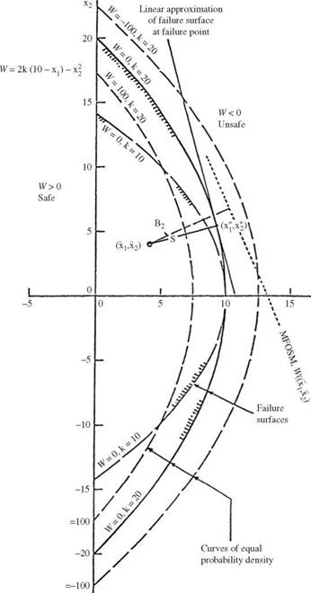
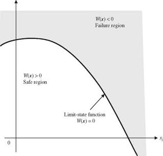
The main thrust of the AFOSM method is to improve the deficiencies associated with the MFOSM method, while keeping the simplicity of the first-order approx­imation. Referring to Fig. 4.3, the difference in the AFOSM method is that the expansion point x+ = (xL*, xR+) for the first-order Taylor series is located on the failure surface defined by the limit-state equation, W(x) = 0. In other words, the failure surface is the boundary that separates the system performance from being unsatisfactory (unsafe) or being satisfactory (safe), that is,

{

> 0, system performance is satisfactory (or safe region);

= 0, limit-state surface (or failure surface);

< 0, system performance is unsatisfactory (or failure region).

The AFOSM method has been applied to various hydrosystem engineering prob­lems, including storm sewers (Melching and Yen, 1986), dams (Cheng et al., 1982; 1993), sea dikes and barriers (Vrijling, 1987; 1993), freeboard design (Cheng et al., 1986a), bridge scour (Yen and Melching, 1991; Chang, 1994), rainfall-runoff modeling (Melching et al., 1990; Melching, 1992); groundwater pollutant transport (Sitar et al., 1987; Jang et al., 1990), open channel design (Easa, 1992), sediment transport (Bechtler and Maurer, 1992), backwater com­putations (Cesare, 1991; Singh and Melching, 1993), and water quality model­ing (Tung, 1990; Melching and Anmangandla, 1992; Melching and Yoon, 1996; Han et al., 2001; Tolson et al., 2001).

4.1.1 Definitions of stochastic parameter spaces

Before discussing the AFOSM methods, a few notations with regard to the stochastic basic variable space are defined first. In general, the original

stochastic basic variables X could be correlated, non-normal random variables having a vector of mean ix = (pxi, /гХ2,…, pxK)t and covariance matrix Cx as shown in Sec. 2.7.2. The original random variables X can be standardized as

X’ = D-1/2(X – fix) (4.30)

in which X’ = (X^, X2,…, XK)t is a vector of correlated, standardized random variables, and Dx = diag(o2, a|,…, oK) is an K x K diagonal variance matrix. Through the standardization procedure, each standardized variable X’ has the mean zero and unit standard deviation. The covariance matrix of X’ reduces to the correlation matrix of the original random variables X, that is, Cx> = Rx, as shown in Sec. 2.7.2. Note that if the original random variables X are nonnormal, the standardized ones X’ are nonnormal as well. Because it is generally easier to work with the uncorrelated variables in the reliability analysis, the correlated random variables X are often transformed into uncorrelated ones U = T (X), with T ( ) representing transformation, in general. More specifically, orthogonal transforms often are used to obtain uncorrelated random variables from the correlated ones. Two frequently used orthogonal transforms, namely, Cholesky decomposition and spectral decomposition, for dealing with correlated random variables are described in Appendix 4B. In probability evaluation, it is generally convenient to deal with normal random variables. For this reason, orthogonal transformation, normal transformation, and standardization procedures are applied to the original random variables X to obtain independent, standardized normal random variables Z’. Hence this chapter adopts X for stochastic basic variables in the original scale, X’ for the standardized correlated stochastic basic variables, U for the uncorrelated variables, and Z and Zrespectively, for correlated and independent, standardized normal stochastic basic variables.

Mean-Value First-Order Second-Moment (MFOSM) Method

In the first-order methods, the performance function W (X), defined on the basis of the loading and resistance functions g(XL) and h(XR), are expanded in a Taylor series at a reference point. The second – and higher-order terms in the series expansion are truncated, resulting in an approximation involving only the first two statistical moments of the variables. This simplification greatly en­hances the practicality of the first-order methods because, in many problems, it is rather difficult, if not impossible, to find the PDF of the variables, whereas it is relatively simple to estimate the first two statistical moments. The pro­cedure is based on the first-order variance estimation (FOVE) method, which is summarized below. For a detailed description of the method in uncertainty analysis, readers are referred to Tung and Yen (2005, Sec. 5.1).

Mean-Value First-Order Second-Moment (MFOSM) Method

The first-order variance estimation (FOVE) method, also called the vari­ance propagation method (Berthouex, 1975), estimates uncertainty features of a model output based on the statistical properties of the model’s stochas­tic basic variables. The basic idea of the method is to approximate a model involving stochastic basic variables by a Taylor series expansion. Consider that a hydraulic or hydrologic performance function W (X) is related to K stochastic basic variables because W(X) = W(X1,X2,…,XK), in which X = (X1, X 2,…, XK )t, a K-dimensional column vector of variables in which all Xs are subject to uncertainty, the superscript t represents the transpose of a matrix or vector. The Taylor series expansion of the performance function W (X) with respect to a selected point of stochastic basic variables X = xo in the parameter space can be expressed as

in which wo = W(xo), and є represents the higher-order terms. The partial derivative terms are called sensitivity coefficients, each representing the rate of change in the performance function value W with respect to the unit change of the corresponding variable at xo.

Dropping the higher-order terms represented by є, Eq. (4.19) is a second – order approximation of the model W(X). Further truncating the second-order terms from it leads to the first-order approximation of W as

Mean-Value First-Order Second-Moment (MFOSM) Method

K


d W (X)
d Xk


W (X)


(Xk xko)


(4.20)


x


k=1


or in a matrix form as

Подпись: (4.21)W (X) = wo + sO (X – x o)

Подпись: and Mean-Value First-Order Second-Moment (MFOSM) Method

where sO = VxW(xo) is the column vector of sensitivity coefficients with each element representing dW/дXk evaluated at X = xO. The mean and variance of W by the first-order approximation can be expressed, respectively, as

Подпись: and Подпись: {Aw & wo + So (Mx x o ) aw & So Cx so Подпись: (4.24) (4.25)

In matrix forms, Eqs. (4.22) and (4.23) can be expressed as

in which fix and Cx are the vectors of the means and covariance matrix of the stochastic basic variables X, respectively.

Commonly, the first-order variance estimation method consists of taking the expansion point xo = (Ax at which the mean and variance of W reduce to

{Aw & g(Mx) — w (4.26)

and aw & s*CxS (4.27)

in which s = Vx W(p, x) is a K-dimensional vector of sensitivity coefficients eval­uated at xo = fAx. When all stochastic basic variables are independent, the variance of model output W could be approximated as

K

aw ^2 skal =s * Dxs (4.28)

k=1

in which Dx = diag(a12, af,…, aK)isaK x K diagonal matrix of variances of the involved stochastic basic variables. From Eq. (4.28), the ratio sak/Var( W) indi­cates the proportion of the overall uncertainty in the model output contributed by the uncertainty associated with the stochastic basic variable Xk.

The MFOSM method for reliability analysis first applies the FOVE method to estimate the statistical moments of the performance function W (X). This is done by applying the expectation and variance operators to the first-order Taylor series approximation of the performance function W (X) expanded at the mean values of the stochastic basic variables. Once the mean and stan­dard deviations of W (X) are estimated, the reliability is computed according to Eqs. (4.9) or (4.10), with the reliability index ^MFOSM computed as

Amfosm = , (4.29)

Vs1 Cx s

where fxx and Cx are the vectors of means and covariance matrix of stochas­tic basic variables X, respectively, and s = VxW(px) is the column vector of sensitivity coefficients with each element representing d W/дXk evaluated at X = l^x.

Example 4.6 Manning’s formula for determining flow capacity of a storm sewer is

Q = 0.463n—1 D267 S 05

in which Q is flow rate (in ft3/s), n is the Manning roughness coefficient, D is the sewer diameter (in ft), and S is pipe slope (in ft/ft). Because roughness coefficient n, sewer diameter D, and sewer slope S in Manning’s formula are subject to uncertainty owing to manufacturing imprecision and construction error, the sewer flow capacity would be subject to uncertainty. Consider a section of circular sewer pipe with the following features:

Model parameter

Nominal value

Coefficient of variation

Roughness coefficient (n)

0.015

0.05

Pipe diameter (D, ft.)

3.0

0.05

Pipe slope (S, ft/ft)

0.005

0.05

Compute the reliability that the sewer capacity could convey a discharge of 35 ft3/s. Assume that stochastic model parameters n, D, and S are uncorrelated.

Solution The performance function for the problem is W = Q — 35 = 0.463n-1 D267 S0 5 — 35. The first-order Taylor series expansion of the performance function about no = xn = 0.015, Do = xd = 3.0, and So = xs = 0.005, according to Eq. (4.20), is

W ^ 0.463(0.015)—1(3)2’67(0.005)°’5 + (9Q/дn)(n — 0.015) + (9Q/дD)(D — 3.0)

+ (9 Q/д S )(S — 0.0005) — 35

= 41.01 — 2733.99(n — 0.015) + 36.50( D — 3.0) + 4100.99( S — 0.005) — 35 Based on Eq. (4.26), the approximated mean of the sewer flow capacity is

Xw ^ 41.01 — 35 = 6.01 ft3/s

Owing to independency of n, D, and S, according to Eq. (4.28), the approximated variance of the performance function W is

oQ ъ (2733.99)[6]Var(n) + (36.50)2Var(D) + (4100.99)2Var(S)

Since

Var(n) = (QnM-n)2 = (0.05 x 0.015)2 = (7.5 x 10—4)2 Var(D) = (QDjxD)2 = (0.05 x 3.0)2 = (1.5 x 10⁻¹)2 Var(S) = (QS/xS)2 = (0.05 x 0.005)2 = 0.000252 = 6.25 x 10—8 the variance of the performance function W can be computed as

oQ ъ (2733.99)2(7.5 x 10—4)2 + (36.50)2(1.5 x 10⁻¹)2 + (4100.99)2(2.5 x 10—4)2 = 2.052 + 5.472 + 1.032 = 35.23(ft[7]/s)2

Hence the standard deviation of the sewer flow capacity is V35.23 = 5.94 ft3/s.

The MFOSM reliability index is ^mfosm = 6.01/5.94 = 1.01. Assuming a normal distribution for Q, the reliability that the sewer capacity can accommodate a discharge of 35 ft3/s is

Ps = P [Q > 35] = $(^mfosm) = Ф(1.01) = 0.844 The corresponding failure probability is pf = Ф( —1.01) = 0.156.

Yen and Ang (1971), Ang (1973), and Cheng et al. (1986b) indicated that provided that ps < 0.99, reliability is not greatly influenced by the choice of distribution for W, and the assumption of a normal distribution is satisfactory. However, for reliability higher than this value (for example, ps = 0.999), the shape of the tail of a distribution becomes very critical. In such cases, accurate assessment of the distribution of W (X) should be used to evaluate the reliability or failure probability. The MFOsM method has been used widely in various hydrosystems infrastructural designs and analyses such as storm sewers (Tang and Yen, 1972; Tang et al., 1975; Yen and Tang, 1976; Yen et al., 1976), culverts (Yen et al., 1980; Tung and Mays, 1980), levees (Tung and Mays, 1981; Lee and Mays, 1986), floodplains (McBean et al., 1984), and open-channel hydraulics (Huang, 1986).

Example 4.7 Referring to Example 4.6, using the same values of the mean and stan­dard deviation for sewer flow capacity, the following table lists the reliabilities and failure probabilities determined by different distributional assumptions for the sewer flow capacity Q to accommodate the inflow discharge of 35 ft3/s.

Distribution

Ps

Pf

Normal

0.996955

0.003045

Lognormal

0.997704

0.002296

Gumbel

0.999819

0.000191

As can be seen, using different distributional assumptions might result in signifi­cant differences in the estimation of failure probability. This results mainly from the fact that the MFOSM method solely uses the first two moments without taking into account the distributional properties of the random variables.

Assuming that stochastic parameters in the sewer capacity formula (that is, n, D, and S) are uncorrelated lognormal random variables, the sewer capacity also is a lognormal random variable. The following table lists the values of the exact reliabil­ity index and failure probability and those obtained from the MFOSM by Eq. (4.29) and (4.8). The table indicates that approximation by the MFOSM becomes less and less accurate as the computation approaches the tail portion of the distribution.

Inflow rate (ft3/s)

MFOSM

Exact

в1

pf = Ф(-0Р

в2

pf = Ф(-в2)

25

5.035

2.384 x 10⁻⁷

6.350

» 0

30

3.457

2.728 x 10⁻⁴

3.991

3.290 x 10⁻⁵

35

1.880

3.045 x 10⁻³

1.996

2.296 x 10⁻³

40

0.303

3.810 x 10⁻¹

0.268

3.943 x 10⁻¹

45

-1.274

8.988 x 10⁻¹

-1.256

8.954 x 10⁻¹

NOTE: 01 = ixw/aw, 02 = MlnwMnw, and W = Q – inflow.

Application of the MFOSM method is simple and straightforward. However, it possesses certain weaknesses in addition to the difficulties with accurate es­timation of extreme failure probabilities mentioned earlier. These weaknesses include [8] 2 3

Mean-Value First-Order Second-Moment (MFOSM) Method

Figure 4.3 Differences in expansion points and reliability indices between the MFOSM and AFOSM methods.

TABLE 4.2 Effect of Skewness on the Accuracy of p Estimated by the MFOSM Method

Ow

^w

Yw

Exact

MFOSM

eExact

pf

eMFOSM

pf

1.0

0.3

0.3

0.927

7.70

7.036 x 10⁻¹⁵

3.00

1.350 x 10⁻³

1.0

0.5

0.5

1.625

4.64

1.759 x 10⁻⁶

1.80

3.593 x 10⁻²

1.0

1.0

1.0

4.000

2.35

9.402 x 10⁻³

0.90

1.841 x 10⁻¹

1.0

2.0

2.0

27.00

1.18

1.190 x 10⁻¹

0.45

3.260 x 10⁻¹

NOTE: pf = P(W < 0.1), with W being a lognormal random variable.

of the original performance function. In case the performance function is highly nonlinear, linear approximation of such a nonlinear function will not be accurate. Consequently, the estimations of the mean and variance of a nonlinear performance function will be less accurate. The accuracy asso­ciated with the estimated mean and variance deteriorates rapidly as the degree of nonlinearity of the performance function increases. For a linear performance function, the FOVE method would produce the exact values for the mean and variance.

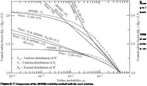
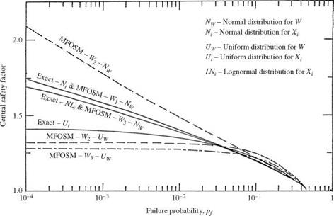
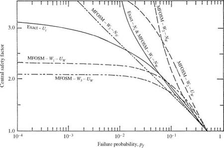
4. Sensitivity of the computed failure probability to the formulation of the per­formance function W. Ideally, the computed reliability or failure probabil­ity for a system should not depend on the definition of the performance function. However, this is not the case for the MFOSM method. This phe­nomenon of lack of invariance to the type of performance function is shown in Figs. 4.4 and 4.5. The main reason for this inconsistency is because the MFOSM method would result in different first-order approximations for dif­ferent forms of the performance function. Consequently, different values of mean and variance will be obtained, resulting in different estimations of re­liability and failure probability for the same problem. This behavior of the MFOSM could create an unnecessary puzzle for engineers with regard to which performance function should be used to obtain an accurate estimation of reliability. This is not an easy question to answer, in general, except for a very few simple cases. Another observation that can be made from Figs. 4.4 and 4.5 is that the discrepancies among failure probabilities computed by the MFOSM method using different performance functions become more pronounced as the uncertainties of the stochastic basic variables get larger.

5. Limited ability to use available probabilistic information. The reliability index в gives only weak information on the probability of failure, and thus the appropriate system probability distribution must be assumed. Further, the MFOSM method provides no logical way to include available information on basic variable probability distributions.

From these arguments, the general rule of thumb is not to rely on the result

of the MFOSM method if any of the following conditions exist: (1) high accuracy

Mean-Value First-Order Second-Moment (MFOSM) Method

Figure 4.4 Comparison of risk-safety factor curves by different methods using various distributions with &L = = 0.1, where Wj = R — L, W2 = (R/L) — 1, and W3 = ln(R/L), and R is the

resistance of the system and L is the load placed on the system. (After Yen et al., 1986.)

Mean-Value First-Order Second-Moment (MFOSM) Method

Figure 4.5 Comparison of risk-safety factor curves by different methods using various distri­butions with &L = &R = 0.3, where Wj = R — L, W2 = (R/L) — 1, and W3 = ln(R/L), and R is the resistance of the system and L is the load placed on the system. (After Yen et al., 1986.)

requirement for the estimated reliability or failure probability, (2) high non­linearity of the performance function, and (3) many skewed random variables involved in the performance function. However, Cornell (1969) made a strong defense for the MFOSM method from a practical standpoint as follows:

An approach based on means and variances may be all that is justified when one appreciates (1) that data and physical arguments are often insufficient to establish the full probability law of a variable; (2) that most engineering analyses include an important component of real, but difficult to measure, professional uncertainty; and (3) that the final output, namely, the decision or design parameters, is often not sensitive to moments higher than the mean and variance.

To reduce the effect of nonlinearity, one way is to include the second-order terms in the Taylor series expansion. This would increase the burden of analysis by having to compute the second-order partial derivatives. Another alternative within the realm of first-order simplicity is given in Sec. 4.5. Section 4.6 briefly describes the basis of the second-order reliability analysis techniques.

Direct Integration Method

Direct Integration Method Подпись: dr dt Подпись: (4.11a) (4.11b)

From Eqs. (4.1) and (4.4) one realizes that the computation of reliability requires knowledge of the probability distributions of the load and resistance or of the performance function W. In terms of the joint PDF of the load and resistance, Eq. (4.1) can be expressed as

Direct Integration Method Подпись: (4.12a) (4.12b)

in which f R L(r, t) is the joint PDF of random load L and resistance R, r and t are dummy arguments for the resistance and load, respectively, and (r1, r2) and (t1, t2) are the lower and upper bounds for the resistance and load, respectively. The failure probability can be computed as

This computation of reliability is commonly referred to as load-resistance interference.

Подпись: 150

TABLE 4.1 Reliability Formulas for Selected Distributions


Distribution
of W


Coefficient of

variation Reliability ps — P (W > 0)


Probability density function fw(w)


Mean


Direct Integration Method

Ow


Normal


Ф


°wl^w


2


МГп w Oln w


Direct Integration Method

vaw-1


Lognormal


Ф


Direct Integration Method

1

1 + в wo


g-fti-w-wo)


Exponential


Direct Integration Method

1 – IG[a, в(w – $)]| Г(а)*


Gamma


a + в$


Bu (a, в)t
B(a, в)


а

a^—– (b — a)

a + в


ав


(b – a)


Direct Integration Method

Beta


a + в + 1 (a + в)^и


Direct Integration Method

Triangular


for a w m


/ 1/2 /1 ab + am + bm

V2 6^w J


a + m + b

3


_ (b – w)2

(b – a)(b – m) for m < w < b

b – w b-a


for m w b


1 b – a V3 b + a


a + b
2


1


for a < w < b


Uniform


ba


*IG( ) — incomplete gamma function. t Bu(■) — incomplete beta function. SOURCE: After Yen et al. (1986).


Example 4.2 Consider the following joint PDF for the load and resistance: f R, L(r, t) = (r + t + r t)e-(r +t+rt) for r > 0,t > 0

Compute the reliability ps.

Подпись: Ps = Подпись: (r + t + r t)e-(r +t+r t} dt Подпись: dr

Solution According to Eq. (4.11), the reliability can be computed as

/* TO

/ [-(1 + t)e-(r +t+r t) ]0 dr

■J0

e-r – (1 + r )e-(2r +r2)

dr =

1 e-(2r +r2) _ e-r

2

= 0.5

0

When the load and resistance are statistically independent, Eq. (4.11) can be reduced to

Ps = Г2 FL(r) fR(r) dr = Er [Fl(R)] (4.13a)

Jr 1

or Ps ^"2[1 – Fr(t)] fL(t) dt = 1 – El[Fr(L)] (4.13b)

Jt1

in which Fl() and Fr () are the marginal CDFs of random load L and resistance R, respectively, Er [Fl(R)] is the expected value of the CDF of random load over the possible range of the resistance, and El[Fr(L)] is the expected value of the CDF of random resistance over the possible range of the load. Similarly, the failure probability, when the load and resistance are independent, can be expressed as

Pf = 1 – Ps = Er[1 – Fl(R)] = El[Fr(L)] (4.14)

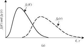
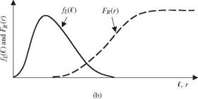
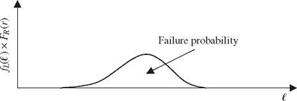
A schematic diagram illustrating load-resistance interference in the reliability computation, when the load and resistance are independent random variables, is shown in Fig. 4.2.

Example 4.3 Consider that the load and resistance are uncorrelated random vari­ables, each of which has the following PDF:

Load (exponential distribution):

f L(t) = 2e-2t for t > 0

Resistance (Erlang distribution):

f r(r) = 4re-2r for r > 0

Compute the reliability Ps.

(c)


fw (w)

Direct Integration Method

Figure 4.2 Schematic diagram of load-resistance interference for computing failure probability: (a) marginal densities of load and resistance; (b) PDF of load and CDF of resistance; (c) compute f L,(i) x Fr(r) over valid range of load; the area underneath the curve is the failure probability; (d) PDF of the performance function; the area left of w = 0 is the failure probability.


Direct Integration MethodDirect Integration MethodDirect Integration Method

Direct Integration Method

Подпись: Ps = / (4re-2r) Jo Direct Integration Method Подпись: dr

Solution Since the load and resistance are uncorrelated random variables, the relia­bility ps can be computed according to Eq. (4.13a) as

Подпись: J Q

/•TO

/ (4re-2r )(1 – e-2r) dr

Jq

1 + r) e-4r – (1 + 2r )e-2r

= 0.75

In the case that the PDF of the performance function W is known or derived, the reliability can be computed according to Eq. (4.4) as

п to

Ps = / fw(w) dw (4.15)

0

in which f w(w) is the PDF of the performance function.

Example 4.4 Define the performance function W = R – L, in which R and L are independent random variables with their PDFs given in Example 4.2. Determine the reliability ps using Eq. (4.15).

Solution To use Eq. (4.15) for the reliability computation, it is necessary to first obtain the PDF of the performance function W. Derivation of the PDF of W can be made based on the derived distribution method described in Tung and Yen (2005, Sec. 3.1) as follows: Define W = R – L and U = L from which the original random variables R and L can be expressed in terms of new random variables W and U as L = U and R = W + U. By the transformation of variables, the joint PDF of W and U can be expressed as

fw, u(w, u) = f R, L(r, t)| J |

Подпись: J =

Подпись: 0 1 1 1

Подпись: - d L dW d R -dW Подпись: d L- dU d R dU-

in which the Jacobian matrix J is

The absolute value of the determinant of the Jacobian matrix | J | is equal to one. Hence the joint PDF of W and U is

fw, u(w, u) = f r(r) fL(t)| J | = f r(w + u) f l(u)(1) = 8(w + u)e 2(w+2u)

Подпись: fw(w) Подпись: PTO fw,u(w, u) du Подпись: 11 + 4w 2 e2w Подпись: for w 0

for – to < w < ж and u > 0. Because the marginal PDF associated with the perfor­mance function W is needed, it can be obtained from the preceding joint PDF as

Подпись: Ps = Подпись: 0 Подпись: 1 + 4w e2w Подпись: dw = Подпись: w+4 Подпись: e Direct Integration Method Подпись: 0.75

From the derived PDF for W, the reliability can be computed as

In the conventional reliability analysis of hydraulic engineering design, un­certainty from the hydraulic aspect often is ignored. Treating the resistance or capacity of the hydraulic structure as a constant reduces Eq. (4.11) to

Ps = l fbU) di (4.16)

0

in which ro is the resistance of the hydraulic structure, a deterministic quan­tity. If the PDF of the hydrologic load is the annual event, such as the annual maximum flood, the resulting annual reliability can be used to calculate the corresponding return period.

Подпись: Ps = Direct Integration Method Direct Integration Method Подпись: (4.17)

To express the reliability in terms of stochastic variables in load and resis­tance functions, Eq. (4.11) can be written as

in which f (xL, xR) is the joint PDF of model stochastic basic variables X. For independent stochastic basic variables X, Eq. (4.17) can be written as

Direct Integration MethodK

П fk (Xk) d xr (4.18)

k=m+1

in which fk ( ) is the marginal PDF of the stochastic basic variable Xk.

The method of direct integration requires the PDFs of the load and resistance or the performance function to be known or derived. This is seldom the case in practice, especially for the joint PDF, because of the complexity of hydrologic and hydraulic models used in design. Explicit solution of direct integration can be obtained for only a few PDFs, as given in Table 4.1 for the reliability ps. For most other PDFs, numerical integration may be necessary. Computation­ally, the direct integration method is analytically tractable for only very few special combinations of probability distributions and functional relationships. For example, the distribution of the safety margin W expressed by Eq. (4.5) has a normal distribution if both load and resistance functions are linear and all stochastic variables are normally distributed. In terms of the safety factor expressed as Eqs. (4.6) and (4.7), the distribution of W (X) is lognormal if both load and resistance functions have multiplicative forms involving lognormal stochastic variables. Most of the time, numerical integrations are performed for reliability determination. When using numerical integration (including Monte Carlo simulation described in Chap. 6), difficulty may be encountered when one deals with a multivariate problem. Appendix 4A summarizes a few one­dimensional numerical integration schemes.

Example 4.5 Referring to Example 4.1, the stochastic basic variables n, D, and S in Manning’s formula to compute the sewer capacity are independent lognormal random variables with the following statistical properties:

Parameter

Mean

Coefficient of variation

n (ft1/6)

0.015

0.05

D (ft)

3.0

0.02

S (ft/ft)

0.005

0.05

Compute the reliability that the sewer can convey the inflow discharge of 35 ft3/s.

Solution In this example, the resistance function is R(n, D, S) = 0.463 n-1 D2 67S0 5, and the load is L = 35 ft3/s. Since all three stochastic parameters are lognormal random variables, the performance function appropriate for use is

W(n, D, S) = ln(R) – ln(L)

= [ln(0.463) – ln(n) + 2.67 ln(D) + 0.5ln(S)] – ln(35)

= — ln(n) + 2.67 ln(D) + 0.5 ln(S) – 4.3319

The reliability ps = P [W(n, D, S) > 0] then can be computed as follows:

Since n, D, and S are independent lognormal random variables, ln(n), ln(D), and ln( S) are independent normal random variables. Note that the performance function W(n, D, S) is a linear function of normal random variables. Then, by the reproductive property of normal random variables as described in Sec. 2.6.1, W(n, D, S) also is a normal random variable with the mean

Pw = – Mln(n) + 2.67Pln(D) + °.5Mln(S) – 4.3319

and the variance

Var( W) = Var[ln(n)] + 2.672Var[ln( D)] + 0.52Var[ln( S)]

From Eq. (2.67), the means and variances of log-transformed variables can be obtained as

Var[ln(n)] = ln(1 + 0.052) = 0.0025 Pln(n) = ln(pn) – 0.5 Var[ln(n)] = -4.201

Var[ln(D)] = ln(1 + 0.022) = 0.0004 Pln(D) = ln(pD) – 0.5 Var[ln(D)] = 1.0984

Var[ln(S)] = ln(1 + 0.052) = 0.0025 Pln(S) = ln(pg) – 0.5 Var[ln(S)] = —5.2996

Then the mean and variance of the performance function W (n, D, S) can be computed as

pw = 0.1517 Var(W) = 0.005977

The reliability can be obtained as

ps = P (W > 0) = Ф f—) = ф( 10,1517 ^ = Ф(1.958) = 0.975 awJ VV0.005977 J

Performance Functions and Reliability Index

In reliability analysis, Eq. (4.3) alternatively can be written in terms of a per­formance function W (X) = W (XL, XR) as

ps = P [W(Xl, Xr) > 0] = P [W(X) > 0] (4.4)

in which X is the vector of basic stochastic variables in the load and resistance functions. In reliability analysis, the system state is divided into the safe (sat­isfactory) set defined by W (X) > 0 and the failure (unsatisfactory) set defined by W (X) < 0 (Fig. 4.1). The boundary that separates the safe set and failure set is a surface, called the failure surface, defined by the function W(X) = 0, called the limit-state function. Since the performance function W(X ) defines the condition of the system, it is sometimes called system-state function.

Xk

Performance Functions and Reliability Index

Figure 4.1 System states defined by performance (limit-state) function.

The performance function W(X) can be expressed differently as

Wi(X) = R – L = h(XR) – g(XL) (4.5)

W2(X) = (R/L) – 1 = [h(Xr)/g(Xl)] – 1 (4.6)

W3(X) = ln(R/L) = ln[h(Xr)] – ln[g(Xl)] (4.7)

Referring to Sec. 1.6, Eq. (4.5) is identical to the notion of a safety margin, whereas Eqs. (4.6) and (4.7) are based on safety factor representations.

Example 4.1 Consider the design of a storm sewer system. The sewer flow-carrying capacity Qc (ft3/s) is determined by Manning’s formula:

Qc = 0463xcD8/3 S1/2 n

where n is Manning’s roughness coefficient, Xc is the model correction factor to account for the model uncertainty, D is the actual pipe diameter (ft), and S is the pipe slope (ft/ft). The inflow Ql (ft3/s) to the sewer is the surface runoff whose peak discharge can be estimated by the rational formula

Ql =кLCiA

in which Xl is the correction factor for model uncertainty, C is the runoff coefficient, i is the rainfall intensity (in/h), and A is the runoff contributing area (acres). In the reliability analysis, the sewer flow-carrying capacity Qc is the resistance, and the peak discharge of the surface runoff Ql is the load. The performance functions can be expressed as one of the following three forms:

W1 = Qc – Ql = 0463XcD8/3S1/2 – XLCiA n

W2 = Qc – 1 = 0463XcD8/3S 1/2x-1C-1i-1 A-1 – 1 2 Ql n c L

W3 = ln ^= ln(0.463) – ln(n) + ln(Xc) + 3 ln(D) + 1 ln(S) – ln(XL)

– ln(C) – ln(i) – ln( A)

Also in the reliability analysis, a frequently used reliability indicator в is called the reliability index. The reliability index was first introduced by Cornell (1969) and later formalized by Ang and Cornell (1974). It is defined as the ratio of the mean to the standard deviation of the performance function W (X), which is the inverse of the coefficient of variation of the performance function W (X),

Подпись:в ___ gw

aw

in which gw and aw are the mean and standard deviation of the performance function, respectively. From Eq. (4.8), assuming an appropriate probability
density function for the random performance function W (X), the reliability then can be computed as

Ps = 1 – Fw(0) = 1 – Fw(-в) (4.9)

in which Fw( ) is the cumulative distribution function of the performance func­tion W, and W’ is the standardized performance function defined as W’ = (W – pw)/aw. The expressions of reliability ps for some distributions of W(X) are given in Table 4.1. For distributions not listed, expressions can be found in Sec. 2.6. For practically all probability distributions used in the relia­bility analysis, the value of the reliability ps is a strictly increasing function of the reliability index в. In practice, the normal distribution is used commonly for W(X), in which case the reliability can be computed simply as

Ps = 1 – Ф(-в) = ф(в) (4.10)

where Ф( ) is the standard normal CDF the table for which is given in Table 2.2. Without using the normal probability table, the value of Ф( ) can be computed by various algebraic formulas described in Sec. 2.6.1.

Reliability Analysis Considering Load-Resistance Interference

4.1 Basic Concept

The design of a hydrosystem involves analyses of flow processes in hydrology and hydraulics. In a multitude of hydrosystems engineering problems, uncer­tainties in data and in theory, including design and analysis procedures, war­rant a probabilistic treatment of the problems. The risk associated with the potential failure of a hydrosystem is the result of the combined effects of in­herent randomness of external loads and various uncertainties involved in the analysis, design, construction, and operational procedures. Hence, to evaluate the probability that a hydrosystem will function as designed requires uncer­tainty and reliability analyses.

As discussed in Sec. 1.5, failure of an engineering system can be defined as the load L (external forces or demands) on the system exceeding the resistance R (strength, capacity, or supply) of the system. The reliability ps is defined as the probability of safe (or nonfailure) operation, in which the resistance of the structure exceeds or equals to the load, that is,

Ps = P (L < R) (4.1)

in which P(■) denotes the probability. Conversely, failure probability pf can be computed as

Pf = P (L > R) = 1 – ps (4.2)

The definitions of reliability and failure probability, Eqs. (4.1) and (4.2), are equally applicable to component reliability, as well as total system

Copyright © 2006 by The McGraw-Hill Companies, Inc. Click here for terms of use.

reliability. In hydrosystems engineering analyses, the resistance and load frequently are functions of several stochastic basic variables, that is, L = g( Xl) = g( X ь X 2,…, Xm) and R = h( Xr ) = h( Xm+1, Xm+2,…, Xk ), where Xі, X2,…, XK are stochastic basic variables defining the load function g(Xl) and the resistance function h(Xr ). Accordingly, the failure probability and reliability are functions of stochastic basic variables, that is,

ps = P [g(Xl) < h(Xr)] (4.3)

Note that the foregoing presentation of load and resistance in reliability anal­ysis should be interpreted in a very general context. For example, in the design and analysis hydrosystems infrastructures, such as urban drainage systems, the load could be the inflow to the sewer system, whereas the resistance is the sewer conveyance capacity; in water quality assessment, the load may be the concentration or mass of pollutant entering the environmental system, whereas the resistance is the permissible pollutant concentration set by water quality regulations; in the economic analysis of a hydrosystem, the load could be the total cost, whereas the resistance is the total benefit.

Evaluation of reliability or failure probability by Eqs. (4.1) through (4.3) does not consider the time-dependent nature of the load and resistance if statistical properties of the elements in Xl and Xr do not change with time. This procedure generally is applied when the performance of the system subject to a single worst-load event is considered. From the reliability computation viewpoint, this is referred to as static reliability analysis.

In general, a hydrosystem infrastructure is expected to serve its designated function over an expected period of time. Engineers frequently are interested in knowing the reliability of the structure over its intended service life. In such circumstances, elements of service period, randomness of load occurrences, and possible change in resistance characteristics over time must be consid­ered. Reliability models incorporating these elements are called time-dependent reliability models (Kapur and Lamberson, 1977; Tung and Mays, 1980; Wen, 1987). Computations of the time-dependent reliability of a hydrosystem infras­tructure initially require the evaluation of static reliability. Sections 4.3 through

4.6 describe methods for static reliability analysis, and Sec. 4.7 briefly describes some basic methods for dealing with the time-dependent nature of reliability analysis.

As discussed in the preceding chapters, the natural randomness of hydro­logic and geophysical variables, such as flood and precipitation, is an important part of the uncertainty in the design of hydrosystems infrastructures. However, other uncertainties also may be significant and should not be ignored. Failure to account for the other uncertainties in the reliability analysis in the past (as discussed in Sec. 1.3) hindered progress in evaluation of failure probability as­sociated with hydrosystems infrastructures. As noted by Cornell (1969) with respect to traditional frequency-based analyses of system safety:

It is important in engineering applications that we avoid the tendency to model only those probabilistic aspects that we think we know how to analyze. It is far better to have an approximated model of the whole problem than an exact model of only a portion of it.

The stationarity assumption

Viessman et al. (1977, p. 158) noted that “usually, the length of record as well as the design life for an engineering project are relatively short compared with ge­ologic history and tend to temper, if not justify, the assumption of stationarity.” On the other hand, Klemes (1986) noted that there are many known causes for nonstationarity ranging from the dynamics of the earth’s motion to human- caused changes in land use. In this context, Klemes (1986) reasons that the notion of a 100-year flood has no meaning in terms of average return period, and thus the 100-year flood is really a reference for design rather than a true reflection of the frequency of an event.

3.9.2 Summary comments

The original premise for the use of hydrologic frequency analysis was to find the optimal project size to provide a certain protection level economically, and the quality of the optimization is a function of the accuracy of the estimated flood level. The preceding discussions in this section have indicated that the accuracy of hydrologic frequency estimates may not be high. For example, Beard (1987) reported that the net result of studies of uncertainties of flood frequency analy­sis is that standard errors of estimated flood magnitudes are very high—on the order of 10 to 50 percent depending on the stream characteristics and amount of data available.

Even worse, the assumptions of hydrologic frequency analysis, namely, stationarity and homogeneous, representative data, and good statistical

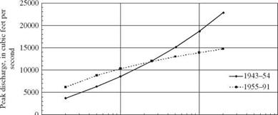
modeling—not extrapolating too far beyond the range of the data—may be violated or stretched in common practice. This can lead to illogical results such as the crossing of pre – and post-change frequency curves illustrated in Fig. 3.8, and the use of such illogical results is based on “a subconscious hope that nature can be cheated and the simple logic of mathematical manipulations can be substituted for the hidden logic of the external world” (Klemes, 1986).

Given the many potential problems with hydrologic frequency analysis, what should be done? Klemes (1986) suggested that if hydrologic frequency theorists were good engineers, they would adopt the simplest procedures and try to stan­dardize them in view of the following facts:

1. The differences in things such as plotting positions, parameter-estimation methods, and even the distribution types, may not matter much in design optimization (Slack et al., 1975). Beard (1987) noted that no matter how reli­able flood frequency estimates are, the actual risk cannot be changed. Thus the benefits from protection essentially are a function of investment and are independent of uncertainties in estimating flood frequencies. Moderate changes in protection or zoning do not change net benefits greatly; i. e., the benefit function has a broad, flat peak (Beard, 1987).

2. There are scores of other uncertain factors in the design that must be settled, but in a rather arbitrary manner, so the whole concept of optimization must be taken as merely an expedient design procedure. The material covered in Chaps. 4, 6, 7, and 8 of this book provide methods to consider the other uncertain factors and improve the optimization procedure.

3. Flood frequency analysis is just one convenient way of rationalizing the old engineering concept of a safety factor rather than a statement of hydrologic truth.

Essentially, the U. S. Water Resources Council (1967) was acting in a manner similar to Klemes’ approach in that a standardized procedure was developed and later improved (Interagency Advisory Committee on Water Data, 1982). However, rather than selecting and standardizing a simple procedure, the rel­atively more complex log-Pearson type 3 procedure was selected. Beard (1987) suggested that the U. S. Water Resources Council methods are the best currently available but leave much to be desired.

Подпись: Problems

Given are the significant independent peak discharges measured on the Saddle River at Lodi, NJ, for two 18-year periods 1948-1965 and 1970-1987. The Saddle River at Lodi has a drainage area of 54.6 mi2 primarily in Bergen County. The total data record for peak discharge at this gauge is as follows: 1924-1937 annual peak only, 1938-1987 all peaks above a specified base value, 1988-1989 annual peak only (data are missing for 1966, 1968, and 1969, hence the odd data periods).

Water

year

Date

Qp (ft3/s)

Water

year

Date

Qp (ft3/s)

Water

year

Date

Qp (ft3/s)

1948

11/09/47

830

1965

2/08/65

8/10/65

1490

1020

1980

3/22/80

4/10/80

4/29/80

1840

2470

2370

1949

12/31/48

1030

1950

3/24/50

452

1951

3/31/51

2530

1970

2/11/70

4/03/70

1770

2130

1981

2/20/81

5/12/81

1540

1900

1952

12/21/51

3/12/52

4/06/52

6/02/52

1090

1100

1470

1740

1971

8/28/71

9/12/71

3530

3770

1982

1/04/82

1980

1983

3/28/83

4/16/83

1800

2550

1972

6/19/72

2240

1953

3/14/53

3/25/53

4/08/53

1860

993

1090

1973

11/09/72

2/03/73

6/30/73

2450

3210

1570

1984

10/24/83

12/13/83

4/05/84

5/30/84

7/07/84

1510

2610

3350

2840

2990

1954

9/12/54

1270

1974

12/21/73

2940

1955

8/19/55

2200

1975

5/15/75

7/14/75

9/27/75

2640

2720

2350

1985

4/26/85

9/27/85

1590

2120

1956

10/16/55

1530

1957

11/02/56

4/06/57

795

795

1976

4/01/76

7/01/76

1590

2440

1986

1/26/86

8/17/86

1850

1660

1958

1/22/58

2/28/58

4/07/58

964

1760

1100

1977

2/25/77

3/23/77

3130

2380

1987

12/03/86

4/04/87

2310

2320

1959

3/07/59

795

1978

11/09/77

1/26/78

3/27/78

4500

1980

1610

1960

9/13/60

1190

1961

2/26/61

952

1962

3/13/62

1670

1979

1/21/79

2/26/79

5/25/79

2890

1570

1760

1963

3/07/63

824

1964

1/10/64

702

3.1 Determine the annual maximum series.

3.2 Plot the annual maximum series on normal, lognormal, and Gumbel probability papers.

3.3 Calculate the first four product moments and L-moments based on the given peak – flow data in both the original and logarithmic scales.

3.4 Use the frequency-factor approach to the Gumbel, lognormal, and log-Pearson type 3 distributions to determine the 5-, 25-, 50-, and 100-year flood peaks.

3.5 Based on the L-moments obtained in Problem 3.3, determine the 5-, 25-, 50-, and 100-year flood peaks using Gumbel, generalized extreme value (GEV), and lognor­mal distributions.

3.6 Determine the best-fit distribution for the annual maximum peak discharge series based on the probability-plot correlation coefficient, the two model relia­bility indices, and L-moment ratio diagram.

3.7 Establish the 95 percent confidence interval for the frequency curve derived based on lognormal and log-Pearson type 3 distribution models.

Extrapolation problems

Most often frequency analysis is applied for the purpose of estimating the mag­nitude of truly rare events, e. g., a 100-year flood, on the basis of short data series. Viessman et al. (1977, pp. 175-176) note that “as a general rule, fre­quency analysis should be avoided… in estimating frequencies of expected hydrologic events greater than twice the record length.” This general rule is followed rarely because of the regulatory need to estimate the 100-year flood; e. g., the U. S. Water Resources Council (1967) gave its blessing to frequency analyses using as few as 10 years of peak flow data. In order to estimate the 100-year flood on the basis of a short record, the analyst must rely on extrap­olation, wherein a law valid inside a range of p is assumed to be valid outside of p. The dangers of extrapolation can be subtle because the results may look plausible in the light of the analyst’s expectations.

The problem with extrapolation in frequency analysis can be referred to as “the tail wagging the dog.” In this case, the “tail” is the annual floods of rela­tively high frequency (1- to 10-year events), and the “dog” is the estimation of extreme floods needed for design (e. g., the floods of 50-, 100-, or even higher-year return periods). When trying to force data to fit a mathematical distribution, equal weight is given to the low end and high end of the data series when trying to determine high-return-period events. Figure 3.6 shows that small changes in the three smallest annual peaks can lead to significant changes in the 100-year peak owing to “fitting properties” of the assumed flood frequency distribution. The analysis shown in Fig. 3.6 is similar to the one presented by Klemes (1986); in this case, a 26-year flood series for Gilmore Creek at Winona, Minnesota, was analyzed using the log-Pearson type 3 distribution employing the skew­ness coefficient estimated from the data. The three lowest values in the annual maximum series (22, 53, and 73 ft3/s) then were changed to values of 100 ft3/s (as if a crest-stage gauge existed at the site with a minimum flow value of 100 ft3/s), and the log-Pearson type 3 analysis was repeated. The relatively small absolute change in these three events changed the skewness coefficient from 0.039 to 0.648 and the 100-year flood from 7,030 to 8,530 ft3/s. As discussed by Klemes (1986), it is illogical that the 1- to 2-year frequency events should have such a strong effect on the rare events.

Under the worst case of hydrologic frequency analysis, the frequent events can be caused by a completely different process than the extreme events. This situation violates the initial premise of hydrologic frequency analysis, i. e., to find some statistical relation between the magnitude of an event and its like­lihood of occurrence (probability) without regard for the physical process of flood formation. For example, in arid and semiarid regions of Arizona, frequent events (1- to 5-year events) are caused by convective storms of limited spa­tial extent, whereas the major floods (> 10-year events) are caused by frontal

Extrapolation problems

1 10 100 Return period, in years

Figure 3.6 Flood frequency analysis for Gilmore Creek at Winona, Minnesota, for 1940-1965 computed with the log-Pearson type 3 distribution fitted to (1) the original annual maximum series and (2) to the original annual maximum series with the three smallest annual peaks set to 100 ft3/s.

monsoon-type storms that distribute large amounts of rainfall over large areas for several days. Figure 3.7 shows the daily maximum discharge series for the Agua Fria River at Lake Pleasant, Arizona, for 1939-1979 and clearly indi­cates a difference in magnitude and mechanism between frequent and infre­quent floods. In this case estimating the 100-year flood giving equal weight in the statistical calculations to the 100 ft3/s and the 26,000 ft3/s flows seems in­appropriate, and an analyst should be prepared to use a large safety factor if standard frequency analysis methods were applied.

Подпись: 0 1 10 100 Return period, in years Figure 3.7 Return periods for the annual maximum daily flow of the Agua Fria River at Lake Pleasant, Arizona, for 1939-1979.
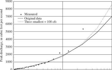
Another problem with “the tail wagging the dog” results when the watershed experiences substantial changes. For example, in 1954 the Vermilion River, Illinois, Outlet Drainage District initiated a major channelization project in­volving the Vermilion River, its North Fork, and North Fork tributaries. The project was completed in the summer of 1955 and resulted in changing the nat­ural 35-ft-wide North Fork channel to a trapezoidal channel 100 ft in width and the natural 75-ft-wide Vermilion channel to a trapezoidal channel 166 ft in width. Each channel also was deepened 1 to 6 ft (U. S. Army Corps of Engineers, 1986). Discharges less than about 8,500 ft3/s at the outlet remain in the modified channel, whereas those greater than 8,500 ft3/s go overbank. At some higher discharge, the overbank hydraulics dominate the flow, just as they did before the channelization. Thus the more frequent flows are increased by the improved hydraulic efficiency of the channel, whereas the infrequent events are still subject to substantial attenuation by overbank flows. Thus the frequency curve is flattened relative to the pre-channelization condition, where the more frequent events are also subject to overbank attenuation. The pre – and post­channelization flood frequency curves cross in the 25- to 50-year return period
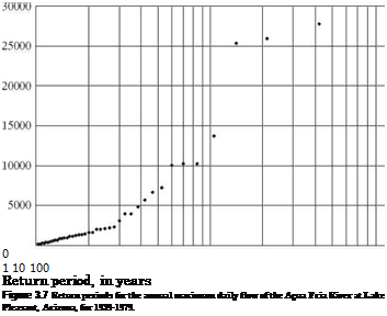
Extrapolation problems

1 10 100 1000

Return period, in years

Figure 3.8 Peak discharge frequency for the Vermilion River at Pontiac, Illinois, for pre-channelized (1943-1954) and post-channelized (1955-1991) conditions.

range (Fig. 3.8), resulting in the illogical result that the pre-channelization condition results in a higher 100-year flood than the post-channelization con­dition. Similar results have been seen for flood flows obtained from continuous simulation applied to urbanizing watersheds (Bradley and Potter, 1991).