Performance Functions and Reliability Index
In reliability analysis, Eq. (4.3) alternatively can be written in terms of a performance function W (X) = W (XL, XR) as
ps = P [W(Xl, Xr) > 0] = P [W(X) > 0] (4.4)
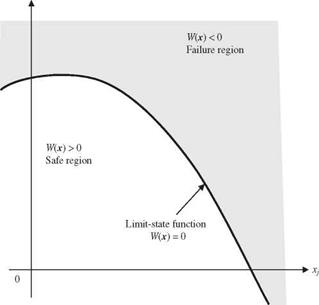
in which X is the vector of basic stochastic variables in the load and resistance functions. In reliability analysis, the system state is divided into the safe (satisfactory) set defined by W (X) > 0 and the failure (unsatisfactory) set defined by W (X) < 0 (Fig. 4.1). The boundary that separates the safe set and failure set is a surface, called the failure surface, defined by the function W(X) = 0, called the limit-state function. Since the performance function W(X ) defines the condition of the system, it is sometimes called system-state function.
|
Xk
Figure 4.1 System states defined by performance (limit-state) function. |
The performance function W(X) can be expressed differently as
Wi(X) = R – L = h(XR) – g(XL) (4.5)
W2(X) = (R/L) – 1 = [h(Xr)/g(Xl)] – 1 (4.6)
W3(X) = ln(R/L) = ln[h(Xr)] – ln[g(Xl)] (4.7)
Referring to Sec. 1.6, Eq. (4.5) is identical to the notion of a safety margin, whereas Eqs. (4.6) and (4.7) are based on safety factor representations.
Example 4.1 Consider the design of a storm sewer system. The sewer flow-carrying capacity Qc (ft3/s) is determined by Manning’s formula:
Qc = 0463xcD8/3 S1/2 n
where n is Manning’s roughness coefficient, Xc is the model correction factor to account for the model uncertainty, D is the actual pipe diameter (ft), and S is the pipe slope (ft/ft). The inflow Ql (ft3/s) to the sewer is the surface runoff whose peak discharge can be estimated by the rational formula
Ql =кLCiA
in which Xl is the correction factor for model uncertainty, C is the runoff coefficient, i is the rainfall intensity (in/h), and A is the runoff contributing area (acres). In the reliability analysis, the sewer flow-carrying capacity Qc is the resistance, and the peak discharge of the surface runoff Ql is the load. The performance functions can be expressed as one of the following three forms:
W1 = Qc – Ql = 0463XcD8/3S1/2 – XLCiA n
W2 = Qc – 1 = 0463XcD8/3S 1/2x-1C-1i-1 A-1 – 1 2 Ql n c L
W3 = ln ^= ln(0.463) – ln(n) + ln(Xc) + 3 ln(D) + 1 ln(S) – ln(XL)
– ln(C) – ln(i) – ln( A)
Also in the reliability analysis, a frequently used reliability indicator в is called the reliability index. The reliability index was first introduced by Cornell (1969) and later formalized by Ang and Cornell (1974). It is defined as the ratio of the mean to the standard deviation of the performance function W (X), which is the inverse of the coefficient of variation of the performance function W (X),
![]() в ___ gw
в ___ gw
in which gw and aw are the mean and standard deviation of the performance function, respectively. From Eq. (4.8), assuming an appropriate probability
density function for the random performance function W (X), the reliability then can be computed as
Ps = 1 – Fw(0) = 1 – Fw(-в) (4.9)
in which Fw( ) is the cumulative distribution function of the performance function W, and W’ is the standardized performance function defined as W’ = (W – pw)/aw. The expressions of reliability ps for some distributions of W(X) are given in Table 4.1. For distributions not listed, expressions can be found in Sec. 2.6. For practically all probability distributions used in the reliability analysis, the value of the reliability ps is a strictly increasing function of the reliability index в. In practice, the normal distribution is used commonly for W(X), in which case the reliability can be computed simply as
Ps = 1 – Ф(-в) = ф(в) (4.10)
where Ф( ) is the standard normal CDF the table for which is given in Table 2.2. Without using the normal probability table, the value of Ф( ) can be computed by various algebraic formulas described in Sec. 2.6.1.


Leave a reply