Mean-Value First-Order Second-Moment (MFOSM) Method
In the first-order methods, the performance function W (X), defined on the basis of the loading and resistance functions g(XL) and h(XR), are expanded in a Taylor series at a reference point. The second – and higher-order terms in the series expansion are truncated, resulting in an approximation involving only the first two statistical moments of the variables. This simplification greatly enhances the practicality of the first-order methods because, in many problems, it is rather difficult, if not impossible, to find the PDF of the variables, whereas it is relatively simple to estimate the first two statistical moments. The procedure is based on the first-order variance estimation (FOVE) method, which is summarized below. For a detailed description of the method in uncertainty analysis, readers are referred to Tung and Yen (2005, Sec. 5.1).
 |
The first-order variance estimation (FOVE) method, also called the variance propagation method (Berthouex, 1975), estimates uncertainty features of a model output based on the statistical properties of the model’s stochastic basic variables. The basic idea of the method is to approximate a model involving stochastic basic variables by a Taylor series expansion. Consider that a hydraulic or hydrologic performance function W (X) is related to K stochastic basic variables because W(X) = W(X1,X2,…,XK), in which X = (X1, X 2,…, XK )t, a K-dimensional column vector of variables in which all Xs are subject to uncertainty, the superscript t represents the transpose of a matrix or vector. The Taylor series expansion of the performance function W (X) with respect to a selected point of stochastic basic variables X = xo in the parameter space can be expressed as
in which wo = W(xo), and є represents the higher-order terms. The partial derivative terms are called sensitivity coefficients, each representing the rate of change in the performance function value W with respect to the unit change of the corresponding variable at xo.
Dropping the higher-order terms represented by є, Eq. (4.19) is a second – order approximation of the model W(X). Further truncating the second-order terms from it leads to the first-order approximation of W as

|
|
||||
|
|
|
|||
|
|||||
|
|||||
or in a matrix form as
![]() W (X) = wo + sO (X – x o)
W (X) = wo + sO (X – x o)
 |
|
where sO = VxW(xo) is the column vector of sensitivity coefficients with each element representing dW/дXk evaluated at X = xO. The mean and variance of W by the first-order approximation can be expressed, respectively, as
 |
||
In matrix forms, Eqs. (4.22) and (4.23) can be expressed as
in which fix and Cx are the vectors of the means and covariance matrix of the stochastic basic variables X, respectively.
Commonly, the first-order variance estimation method consists of taking the expansion point xo = (Ax at which the mean and variance of W reduce to
{Aw & g(Mx) — w (4.26)
and aw & s*CxS (4.27)
in which s = Vx W(p, x) is a K-dimensional vector of sensitivity coefficients evaluated at xo = fAx. When all stochastic basic variables are independent, the variance of model output W could be approximated as
K
aw ^2 skal =s * Dxs (4.28)
k=1
in which Dx = diag(a12, af,…, aK)isaK x K diagonal matrix of variances of the involved stochastic basic variables. From Eq. (4.28), the ratio sak/Var( W) indicates the proportion of the overall uncertainty in the model output contributed by the uncertainty associated with the stochastic basic variable Xk.
The MFOSM method for reliability analysis first applies the FOVE method to estimate the statistical moments of the performance function W (X). This is done by applying the expectation and variance operators to the first-order Taylor series approximation of the performance function W (X) expanded at the mean values of the stochastic basic variables. Once the mean and standard deviations of W (X) are estimated, the reliability is computed according to Eqs. (4.9) or (4.10), with the reliability index ^MFOSM computed as
Amfosm = , (4.29)
Vs1 Cx s
where fxx and Cx are the vectors of means and covariance matrix of stochastic basic variables X, respectively, and s = VxW(px) is the column vector of sensitivity coefficients with each element representing d W/дXk evaluated at X = l^x.
Example 4.6 Manning’s formula for determining flow capacity of a storm sewer is
Q = 0.463n—1 D267 S 05
in which Q is flow rate (in ft3/s), n is the Manning roughness coefficient, D is the sewer diameter (in ft), and S is pipe slope (in ft/ft). Because roughness coefficient n, sewer diameter D, and sewer slope S in Manning’s formula are subject to uncertainty owing to manufacturing imprecision and construction error, the sewer flow capacity would be subject to uncertainty. Consider a section of circular sewer pipe with the following features:
|
Model parameter |
Nominal value |
Coefficient of variation |
|
Roughness coefficient (n) |
0.015 |
0.05 |
|
Pipe diameter (D, ft.) |
3.0 |
0.05 |
|
Pipe slope (S, ft/ft) |
0.005 |
0.05 |
Compute the reliability that the sewer capacity could convey a discharge of 35 ft3/s. Assume that stochastic model parameters n, D, and S are uncorrelated.
Solution The performance function for the problem is W = Q — 35 = 0.463n-1 D267 S0 5 — 35. The first-order Taylor series expansion of the performance function about no = xn = 0.015, Do = xd = 3.0, and So = xs = 0.005, according to Eq. (4.20), is
W ^ 0.463(0.015)—1(3)2’67(0.005)°’5 + (9Q/дn)(n — 0.015) + (9Q/дD)(D — 3.0)
+ (9 Q/д S )(S — 0.0005) — 35
= 41.01 — 2733.99(n — 0.015) + 36.50( D — 3.0) + 4100.99( S — 0.005) — 35 Based on Eq. (4.26), the approximated mean of the sewer flow capacity is
Xw ^ 41.01 — 35 = 6.01 ft3/s
Owing to independency of n, D, and S, according to Eq. (4.28), the approximated variance of the performance function W is
oQ ъ (2733.99)[6]Var(n) + (36.50)2Var(D) + (4100.99)2Var(S)
Since
Var(n) = (QnM-n)2 = (0.05 x 0.015)2 = (7.5 x 10—4)2 Var(D) = (QDjxD)2 = (0.05 x 3.0)2 = (1.5 x 10⁻¹)2 Var(S) = (QS/xS)2 = (0.05 x 0.005)2 = 0.000252 = 6.25 x 10—8 the variance of the performance function W can be computed as
oQ ъ (2733.99)2(7.5 x 10—4)2 + (36.50)2(1.5 x 10⁻¹)2 + (4100.99)2(2.5 x 10—4)2 = 2.052 + 5.472 + 1.032 = 35.23(ft[7]/s)2
Hence the standard deviation of the sewer flow capacity is V35.23 = 5.94 ft3/s.
The MFOSM reliability index is ^mfosm = 6.01/5.94 = 1.01. Assuming a normal distribution for Q, the reliability that the sewer capacity can accommodate a discharge of 35 ft3/s is
Ps = P [Q > 35] = $(^mfosm) = Ф(1.01) = 0.844 The corresponding failure probability is pf = Ф( —1.01) = 0.156.
Yen and Ang (1971), Ang (1973), and Cheng et al. (1986b) indicated that provided that ps < 0.99, reliability is not greatly influenced by the choice of distribution for W, and the assumption of a normal distribution is satisfactory. However, for reliability higher than this value (for example, ps = 0.999), the shape of the tail of a distribution becomes very critical. In such cases, accurate assessment of the distribution of W (X) should be used to evaluate the reliability or failure probability. The MFOsM method has been used widely in various hydrosystems infrastructural designs and analyses such as storm sewers (Tang and Yen, 1972; Tang et al., 1975; Yen and Tang, 1976; Yen et al., 1976), culverts (Yen et al., 1980; Tung and Mays, 1980), levees (Tung and Mays, 1981; Lee and Mays, 1986), floodplains (McBean et al., 1984), and open-channel hydraulics (Huang, 1986).
Example 4.7 Referring to Example 4.6, using the same values of the mean and standard deviation for sewer flow capacity, the following table lists the reliabilities and failure probabilities determined by different distributional assumptions for the sewer flow capacity Q to accommodate the inflow discharge of 35 ft3/s.
|
Distribution |
Ps |
Pf |
|
Normal |
0.996955 |
0.003045 |
|
Lognormal |
0.997704 |
0.002296 |
|
Gumbel |
0.999819 |
0.000191 |
As can be seen, using different distributional assumptions might result in significant differences in the estimation of failure probability. This results mainly from the fact that the MFOSM method solely uses the first two moments without taking into account the distributional properties of the random variables.
Assuming that stochastic parameters in the sewer capacity formula (that is, n, D, and S) are uncorrelated lognormal random variables, the sewer capacity also is a lognormal random variable. The following table lists the values of the exact reliability index and failure probability and those obtained from the MFOSM by Eq. (4.29) and (4.8). The table indicates that approximation by the MFOSM becomes less and less accurate as the computation approaches the tail portion of the distribution.
|
Inflow rate (ft3/s) |
MFOSM |
Exact |
||
|
в1 |
pf = Ф(-0Р |
в2 |
pf = Ф(-в2) |
|
|
25 |
5.035 |
2.384 x 10⁻⁷ |
6.350 |
» 0 |
|
30 |
3.457 |
2.728 x 10⁻⁴ |
3.991 |
3.290 x 10⁻⁵ |
|
35 |
1.880 |
3.045 x 10⁻³ |
1.996 |
2.296 x 10⁻³ |
|
40 |
0.303 |
3.810 x 10⁻¹ |
0.268 |
3.943 x 10⁻¹ |
|
45 |
-1.274 |
8.988 x 10⁻¹ |
-1.256 |
8.954 x 10⁻¹ |
|
NOTE: 01 = ixw/aw, 02 = MlnwMnw, and W = Q – inflow. |
Application of the MFOSM method is simple and straightforward. However, it possesses certain weaknesses in addition to the difficulties with accurate estimation of extreme failure probabilities mentioned earlier. These weaknesses include [8] 2 3
|
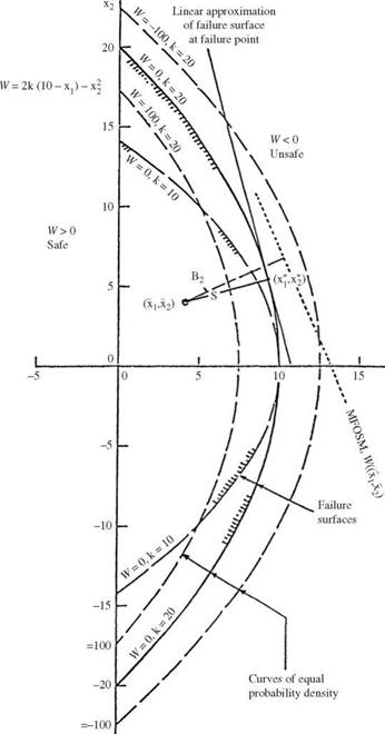
Figure 4.3 Differences in expansion points and reliability indices between the MFOSM and AFOSM methods. |
|
TABLE 4.2 Effect of Skewness on the Accuracy of p Estimated by the MFOSM Method
NOTE: pf = P(W < 0.1), with W being a lognormal random variable. |
of the original performance function. In case the performance function is highly nonlinear, linear approximation of such a nonlinear function will not be accurate. Consequently, the estimations of the mean and variance of a nonlinear performance function will be less accurate. The accuracy associated with the estimated mean and variance deteriorates rapidly as the degree of nonlinearity of the performance function increases. For a linear performance function, the FOVE method would produce the exact values for the mean and variance.
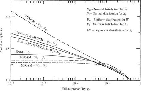
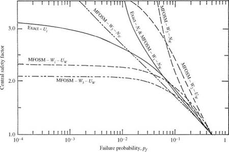
4. Sensitivity of the computed failure probability to the formulation of the performance function W. Ideally, the computed reliability or failure probability for a system should not depend on the definition of the performance function. However, this is not the case for the MFOSM method. This phenomenon of lack of invariance to the type of performance function is shown in Figs. 4.4 and 4.5. The main reason for this inconsistency is because the MFOSM method would result in different first-order approximations for different forms of the performance function. Consequently, different values of mean and variance will be obtained, resulting in different estimations of reliability and failure probability for the same problem. This behavior of the MFOSM could create an unnecessary puzzle for engineers with regard to which performance function should be used to obtain an accurate estimation of reliability. This is not an easy question to answer, in general, except for a very few simple cases. Another observation that can be made from Figs. 4.4 and 4.5 is that the discrepancies among failure probabilities computed by the MFOSM method using different performance functions become more pronounced as the uncertainties of the stochastic basic variables get larger.
5. Limited ability to use available probabilistic information. The reliability index в gives only weak information on the probability of failure, and thus the appropriate system probability distribution must be assumed. Further, the MFOSM method provides no logical way to include available information on basic variable probability distributions.
From these arguments, the general rule of thumb is not to rely on the result
of the MFOSM method if any of the following conditions exist: (1) high accuracy
|
Figure 4.4 Comparison of risk-safety factor curves by different methods using various distributions with &L = = 0.1, where Wj = R — L, W2 = (R/L) — 1, and W3 = ln(R/L), and R is the resistance of the system and L is the load placed on the system. (After Yen et al., 1986.) |
|
Figure 4.5 Comparison of risk-safety factor curves by different methods using various distributions with &L = &R = 0.3, where Wj = R — L, W2 = (R/L) — 1, and W3 = ln(R/L), and R is the resistance of the system and L is the load placed on the system. (After Yen et al., 1986.) |
requirement for the estimated reliability or failure probability, (2) high nonlinearity of the performance function, and (3) many skewed random variables involved in the performance function. However, Cornell (1969) made a strong defense for the MFOSM method from a practical standpoint as follows:
An approach based on means and variances may be all that is justified when one appreciates (1) that data and physical arguments are often insufficient to establish the full probability law of a variable; (2) that most engineering analyses include an important component of real, but difficult to measure, professional uncertainty; and (3) that the final output, namely, the decision or design parameters, is often not sensitive to moments higher than the mean and variance.
To reduce the effect of nonlinearity, one way is to include the second-order terms in the Taylor series expansion. This would increase the burden of analysis by having to compute the second-order partial derivatives. Another alternative within the realm of first-order simplicity is given in Sec. 4.5. Section 4.6 briefly describes the basis of the second-order reliability analysis techniques.


Leave a reply