Direct Integration Method

From Eqs. (4.1) and (4.4) one realizes that the computation of reliability requires knowledge of the probability distributions of the load and resistance or of the performance function W. In terms of the joint PDF of the load and resistance, Eq. (4.1) can be expressed as

in which f R L(r, t) is the joint PDF of random load L and resistance R, r and t are dummy arguments for the resistance and load, respectively, and (r1, r2) and (t1, t2) are the lower and upper bounds for the resistance and load, respectively. The failure probability can be computed as

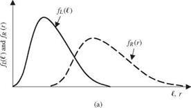
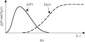
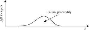
This computation of reliability is commonly referred to as load-resistance interference.

TABLE 4.1 Reliability Formulas for Selected Distributions
Distribution of W
Coefficient of variation Reliability ps — P (W > 0)
Probability density function fw(w)	Mean
Ow
Normal	Ф
°wl^w
2
МГп w Oln w
vaw-1
Lognormal	Ф
1 1 + в wo
g-fti-w-wo)
Exponential
1 — IG[a, в(w — $)]| Г(а)*
Gamma
a + в$
Bu (a, в)t B(a, в)
а a^—— (b — a) a + в	ав	(b — a)
Beta
a + в + 1 (a + в)^и
Triangular	for a w m
/ 1/2 /1 ab + am + bm V2 6^w J
a + m + b 3
_ (b — w)2 (b — a)(b — m) for m < w < b b — w b-a
for m w b
1 b — a V3 b + a
a + b 2
1
for a < w < b
Uniform
ba
*IG( ) — incomplete gamma function. t Bu(■) — incomplete beta function. SOURCE: After Yen et al. (1986).

Example 4.2 Consider the following joint PDF for the load and resistance: f R, L(r, t) = (r + t + r t)e-(r +t+rt) for r > 0,t > 0

Compute the reliability ps.

Solution According to Eq. (4.11), the reliability can be computed as

/* TO

/ [-(1 + t)e-(r +t+r t) ]0 dr

■J0

e-r — (1 + r )e-(2r +r2)	dr =	1 e-(2r +r2) _ e-r
		2

= 0.5

0

When the load and resistance are statistically independent, Eq. (4.11) can be reduced to

Ps = Г2 FL(r) fR(r) dr = Er [Fl(R)] (4.13a)

Jr 1

or Ps ^"2[1 — Fr(t)] fL(t) dt = 1 — El[Fr(L)] (4.13b)

Jt1

in which Fl() and Fr () are the marginal CDFs of random load L and resistance R, respectively, Er [Fl(R)] is the expected value of the CDF of random load over the possible range of the resistance, and El[Fr(L)] is the expected value of the CDF of random resistance over the possible range of the load. Similarly, the failure probability, when the load and resistance are independent, can be expressed as

Pf = 1 — Ps = Er[1 — Fl(R)] = El[Fr(L)] (4.14)

A schematic diagram illustrating load-resistance interference in the reliability computation, when the load and resistance are independent random variables, is shown in Fig. 4.2.

Example 4.3 Consider that the load and resistance are uncorrelated random vari­ables, each of which has the following PDF:

Load (exponential distribution):

f L(t) = 2e-2t for t > 0

Resistance (Erlang distribution):

f r(r) = 4re-2r for r > 0

Compute the reliability Ps.

(c)

fw (w) Figure 4.2 Schematic diagram of load-resistance interference for computing failure probability: (a) marginal densities of load and resistance; (b) PDF of load and CDF of resistance; (c) compute f L,(i) x Fr(r) over valid range of load; the area underneath the curve is the failure probability; (d) PDF of the performance function; the area left of w = 0 is the failure probability.

Solution Since the load and resistance are uncorrelated random variables, the relia­bility ps can be computed according to Eq. (4.13a) as

/•TO

/ (4re-2r )(1 — e-2r) dr

Jq

1 + r) e-4r — (1 + 2r )e-2r

= 0.75

In the case that the PDF of the performance function W is known or derived, the reliability can be computed according to Eq. (4.4) as

п to

Ps = / fw(w) dw (4.15)

0

in which f w(w) is the PDF of the performance function.

Example 4.4 Define the performance function W = R — L, in which R and L are independent random variables with their PDFs given in Example 4.2. Determine the reliability ps using Eq. (4.15).

Solution To use Eq. (4.15) for the reliability computation, it is necessary to first obtain the PDF of the performance function W. Derivation of the PDF of W can be made based on the derived distribution method described in Tung and Yen (2005, Sec. 3.1) as follows: Define W = R — L and U = L from which the original random variables R and L can be expressed in terms of new random variables W and U as L = U and R = W + U. By the transformation of variables, the joint PDF of W and U can be expressed as

fw, u(w, u) = f R, L(r, t)| J |

in which the Jacobian matrix J is

The absolute value of the determinant of the Jacobian matrix | J | is equal to one. Hence the joint PDF of W and U is

fw, u(w, u) = f r(r) fL(t)| J | = f r(w + u) f l(u)(1) = 8(w + u)e 2(w+2u)

for — to < w < ж and u > 0. Because the marginal PDF associated with the perfor­mance function W is needed, it can be obtained from the preceding joint PDF as

From the derived PDF for W, the reliability can be computed as

In the conventional reliability analysis of hydraulic engineering design, un­certainty from the hydraulic aspect often is ignored. Treating the resistance or capacity of the hydraulic structure as a constant reduces Eq. (4.11) to

Ps = l fbU) di (4.16)

0

in which ro is the resistance of the hydraulic structure, a deterministic quan­tity. If the PDF of the hydrologic load is the annual event, such as the annual maximum flood, the resulting annual reliability can be used to calculate the corresponding return period.

To express the reliability in terms of stochastic variables in load and resis­tance functions, Eq. (4.11) can be written as

in which f (xL, xR) is the joint PDF of model stochastic basic variables X. For independent stochastic basic variables X, Eq. (4.17) can be written as

K

П fk (Xk) d xr (4.18)

k=m+1

in which fk ( ) is the marginal PDF of the stochastic basic variable Xk.

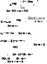
The method of direct integration requires the PDFs of the load and resistance or the performance function to be known or derived. This is seldom the case in practice, especially for the joint PDF, because of the complexity of hydrologic and hydraulic models used in design. Explicit solution of direct integration can be obtained for only a few PDFs, as given in Table 4.1 for the reliability ps. For most other PDFs, numerical integration may be necessary. Computation­ally, the direct integration method is analytically tractable for only very few special combinations of probability distributions and functional relationships. For example, the distribution of the safety margin W expressed by Eq. (4.5) has a normal distribution if both load and resistance functions are linear and all stochastic variables are normally distributed. In terms of the safety factor expressed as Eqs. (4.6) and (4.7), the distribution of W (X) is lognormal if both load and resistance functions have multiplicative forms involving lognormal stochastic variables. Most of the time, numerical integrations are performed for reliability determination. When using numerical integration (including Monte Carlo simulation described in Chap. 6), difficulty may be encountered when one deals with a multivariate problem. Appendix 4A summarizes a few one­dimensional numerical integration schemes.

Example 4.5 Referring to Example 4.1, the stochastic basic variables n, D, and S in Manning’s formula to compute the sewer capacity are independent lognormal random variables with the following statistical properties:

Parameter	Mean	Coefficient of variation
n (ft1/6)	0.015	0.05
D (ft)	3.0	0.02
S (ft/ft)	0.005	0.05

Compute the reliability that the sewer can convey the inflow discharge of 35 ft3/s.

Solution In this example, the resistance function is R(n, D, S) = 0.463 n-1 D2 67S0 5, and the load is L = 35 ft3/s. Since all three stochastic parameters are lognormal random variables, the performance function appropriate for use is

W(n, D, S) = ln(R) — ln(L)

= [ln(0.463) — ln(n) + 2.67 ln(D) + 0.5ln(S)] — ln(35)

= — ln(n) + 2.67 ln(D) + 0.5 ln(S) — 4.3319

The reliability ps = P [W(n, D, S) > 0] then can be computed as follows:

Since n, D, and S are independent lognormal random variables, ln(n), ln(D), and ln( S) are independent normal random variables. Note that the performance function W(n, D, S) is a linear function of normal random variables. Then, by the reproductive property of normal random variables as described in Sec. 2.6.1, W(n, D, S) also is a normal random variable with the mean

Pw = — Mln(n) + 2.67Pln(D) + °.5Mln(S) — 4.3319

and the variance

Var( W) = Var[ln(n)] + 2.672Var[ln( D)] + 0.52Var[ln( S)]

From Eq. (2.67), the means and variances of log-transformed variables can be obtained as

Var[ln(n)] = ln(1 + 0.052) = 0.0025 Pln(n) = ln(pn) — 0.5 Var[ln(n)] = -4.201

Var[ln(D)] = ln(1 + 0.022) = 0.0004 Pln(D) = ln(pD) — 0.5 Var[ln(D)] = 1.0984

Var[ln(S)] = ln(1 + 0.052) = 0.0025 Pln(S) = ln(pg) — 0.5 Var[ln(S)] = —5.2996

Then the mean and variance of the performance function W (n, D, S) can be computed as

pw = 0.1517 Var(W) = 0.005977

The reliability can be obtained as

ps = P (W > 0) = Ф f—) = ф( 10,1517 ^ = Ф(1.958) = 0.975 awJ VV0.005977 J