Selection of Distribution Model

Based on a given sample of finite observations, procedures are needed to help identify the underlying distribution from which the random samples are drawn. Several statistical goodness-of-fit procedures have been developed (D’Agostino and Stephens, 1986). The insensitivity to the tail portion of the distribution of the conventional chi-square test and Kolmogorov-Smirnov test has been well known. Other more powerful goodness-of-fit criteria such as the probability plot correlation coefficient (Filliben, 1975) have been investigated and advocated (Vogel and McMartin, 1991). This and other criteria are described herein.

3.7.1 Probability plot correlation coefficients

The probability plot is a graphic representation of the mth-order statistic of the sample x(m) as a function of a plotting-position F (x(m)). For each order statistic X(m), a plotting-position formula can be applied to estimate its corresponding nonexceedance probability F (X(m>), which, in turn, is used to compute the corre­sponding quantile Ym = G—1[F(X(m>)] according to the distribution model G( ) under consideration. Based on a sample with n observations, the probability plot correlation coefficient (PPCC) then can be defined mathematically as

where ym is the quantile value corresponding to F (x(m)) from a selected plotting — position formula and an assumed distribution model G(-), that is, ym = G-1 [F (x(m))]. It is intuitively understandable that if the samples to be tested are actually generated from the hypothesized distribution model G( ), the corre­sponding plot of X(m) versus ym would be close to linear. The values of F (x(m>) for calculating ym in Eq. (3.17) can be determined by using either a probability — or quantile-unbiased plotting-position formula. The hypothesized distribution model G( ) that yields the highest value of the PPCC should be chosen.

Critical values of the PPCCs associated with different levels of significance for various distributions have been developed. They include normal and lognormal distribution (Fillben, 1975; Looney and Gulledge, 1985; Vogel, 1986), Gumbel distribution (Vogel, 1986), uniform and Weibull distributions (Vogel and Kroll, 1989), generalized extreme-value distribution (Chowdhury et al., 1991), Pear­son type 3 distribution (Vogel and McMartin, 1991), and other distributions (D’Agostino and Stephens, 1986). A distribution is accepted as the underlying random mechanism with a specified significance level if the computed PPCC is larger than the critical value for that distribution.

3.7.2 Model reliability indices

Based on the observed (X(m>} and the computed {ym}, the degree of goodness of fit also can be measured by two reliability indices proposed by Leggett and Williams (1981). They are the geometric reliability index KG,

(3.18)

and the statistical reliability index KS,

When the computed series {ym} perfectly matches with the observed sequence {x(m)}, the values of KG and KS reach their lower bound of 1.0. As the discrep­ancy between {x(m)} and {ym} increases, the values of KG and KS increase. Again, for each of KG and KS, two different values can be computed, each associated with the use of probability-unbiased and quantile-unbiased plotting-position formulas. The most suitable probability model is the one that is associated with the smallest value of the reliability index.

3.7.3 Moment-ratio diagrams

Relationships between product moments and the parameters of various distri­butions are shown in Table 3.4, which also can be found elsewhere (Patel et al., 1976; Stedinger et al., 1993). Similarly, the product-moment ratio diagram
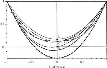
based on skewness coefficient and kurtosis (Stuart and Ord, 1987, p. 211) can be used to identify the distributions. When sample data are used, sample prod­uct moments are used to solve for the model parameters. However, owing to the low reliability of sample skewness coefficient and kurtosis, use of the product — moment ratio diagram for model identification is not reliable. Alternatively, the L-moment ratio diagram defined in the (r3, r4)-space (Fig. 3.3) also can be used for model identification. Namely, one can judge the closeness of the sam­ple L-skewness coefficient and L-kurtosis with respect to the theoretical r3 — r4 curve associated with different distribution models. Some types of distance mea­sures can be computed between the sample point of (t3, t4) and each theoretical т3 — t4 curve. One commonly used distance measure is to compute the shortest distance or distance in L-kurtosis direction fixed at the sample L-skewness coefficient (Pandey et al., 2001). Although it is computationally simple, the

£ —
E Exponential G Gumbel L Logistic N Normal U Uniform	Generalized logistic _ _ Lower bound Generalized extreme-value for wakeby Generalized pareto Lognormal.. Lower bound for Gamma all distributions
T4 Figure 3.3 L-moment ratio diagram and shortest distance from a sample point.

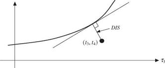
distance measure could not account for the sampling error in the sample L — skewness coefficient. To consider the effect of sampling errors in both the sam­ple L-skewness coefficient and L-kurtosis, the shortest distance between the sample point (t3, t4) and the theoretical r3 — r4 curve of each candidate distribu­tion model is computed for the measure of goodness of fit. The computation of the shortest distance requires locating a point on the theoretical т3 — t4 curve that minimizes the distance as

DIS = min J(t3 — T3)2 + [t4 — t4(t3)]2 (3.20)

T3

Since the theoretical t3 — t4 curve for a specified distribution is unique, determination of the shortest distance was accomplished by an appropriate one­dimensional search technique such as the golden-section procedure or others.

Example 3.7 (Goodness of Fit) Referring to the flood data given in Example 3.3, calculate the values of the probability-unbiased PPCCs and the two reliability indices with respect to the generalized Pareto distribution (GPA).

Solution Referring to Table 3.4, the GPA quantile can be obtained easily as

x(F) = § + в [1 — (1 — F )a]

a

According to the model parameter values obtained from Example 3.6, that is, a = 1.154, в = 361.36, § = 314.64, the GPA quantile can be computed as

x(F) = 314.64 + 36136 [1 — (1 — F)L154]

Using the probability-unbiased plotting position, i. e., the Weibull formula, the cor­responding GPA quantiles are calculated and shown in column (4) of the following table. From data in columns (2) and (4), the correlation coefficient can be obtained as 0.9843.

To calculate the two-model reliability indices, the ratios of GPA quantiles ym to the order flow q(m) are calculated in column (5) and are used in Eqs. (3.18) and (3.19) for Kg and Ks, respectively, as 1.035 and 1.015.

Rank (m) (1)	Ordered q(m) (2)	F (q(m)) = m/(n + 1) (3)	Ут (4)	ym/q(m) (5)
1	342	0.0625	337.1	0.985714
2	374	0.1250	359.4	0.960853
3	390	0.1875	381.4	0.977846
4	414	0.2500	403.1	0.973676
5	416	0.3125	424.6	1.020591
6	447	0.3750	445.7	0.997162
7	505	0.4375	466.6	0.923907
8	505	0.5000	487.1	0.964476
9	507	0.5625	507.2	1.000308
10	524	0.6250	526.8	1.005368
11	533	0.6875	546.0	1.024334
12	543	0.7500	564.5	1.039672
13	549	0.8125	582.4	1.060849
14	591	0.8750	599.4	1.014146
15	596	0.9375	615.0	1.031891

3.7.4 Summary

As the rule for selecting a single distribution model, the PPCC-based criterion would choose the model with highest values, whereas the other two criteria (i. e., reliability index and DIS) would select a distribution model with the smallest value. In practice, it is not uncommon to encounter a case where the values of the adopted goodness-of-fit criterion for different distributions are compatible, and selection of a best distribution may not necessarily be the best course of action, especially in the presence of sampling errors. The selection of acceptable distributions based on the their statistical plausibility through hypothesis test­ing, at the present stage, can only be done for the PPCCs for which extensive experiments have been done to define critical values under various significance levels (or type I errors) and different distributions.