Types of Geophysical Data Series

The first step in the frequency-analysis process is to identify the set of data or sample to be studied. The sample is called a data series because many events of interest occur in a time sequence, and time is a useful frame of reference. The events are continuous, and thus their complete description as a function of time would constitute an infinite number of data points. To overcome this, it is customary to divide the events into a series of finite time increments and con­sider the average magnitude or instantaneous values of the largest or smallest within each interval. In frequency analysis, geophysical events that make up the data series generally are assumed to be statistically independent in time. In the United States, the water year concept was developed to facilitate the independence of hydrologic flood series. Throughout the eastern, southern, and Pacific western areas of the United States, the season of lowest stream flow is late summer and fall (August-October) (U. S. Department of Agriculture, 1955). Thus, by establishing the water year as October 1 to September 30, the chance of having related floods in each year is minimized, and the assumption of independence in the flood data is supported. In case time dependence is present in the data series and should be accounted for, procedures developed in time series analysis (Salas et al., 1980; Salas, 1993) should be applied. This means that the events themselves first must be identified in terms of a beginning and an end and then sampled using some criterion. Usually only one value from each event is included in the data series. There are three basic types of data series extractable from geophysical events:

1. A complete series, which includes all the available data on the magnitude of a phenomenon. A complete data series is used most frequently for flow — duration studies to determine the amount of firm power available in a pro­posed hydropower project or to study the low-flow behavior in water quality management. Such a data series is usually very large, and since in some in­stances engineers are only interested in the extremes of the distribution (e. g., floods, droughts, wind speeds, and wave heights), other data series often are more practical. For geophysical events, data in a complete series often exhibit significant time dependence, which makes the frequency-analysis procedure described herein inappropriate.

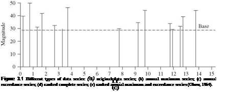
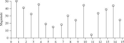
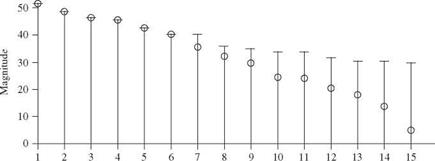
2. An extreme-value series is one that contains the largest (or smallest) data value for each of a number of equal time intervals. If, for example, the largest data value in each year of record is used, the extreme-value series is called an annual maximum series. If the smallest value is used, the series is called an annual minimum series.

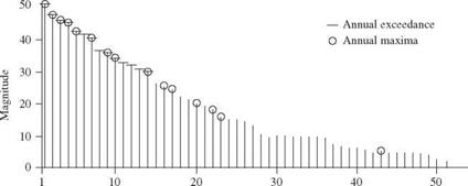
3. A partial-duration series consists of all data above or below a base value. For example, one might consider only floods in a river with a magnitude greater than 1,000 m3/s. When the base value is selected so that the number of events included in the data series equals the number of years of record, the resulting series is called an annual exceedance series. This series contains the n largest or n smallest values in n years of record.

The selection of geophysical data series is illustrated in Fig. 3.1. Figure 3.1a represents the original data; the length of each line indicates the magnitude of the event. Figure 3.16 shows an annual maximum series with the largest data value in each year being retained for analysis. Figure 3.1c shows the data values that would be included in an annual exceedance series. Since there are 15 years of record, the 15 largest data values are retained. Figure 3.1d and e illustrate for comparison the rank in descending order of the magnitude of the events in each of the two series. As shown in Fig. 3.1d and e the annual maximum series and the annual exceedance series form different probability distributions, but when used to estimate extreme floods with return periods of 10 years or more, the differences between the results from the two series are minimal, and the annual maximum series is the one used most commonly. Thus this chapter focuses on the annual maximum series in the following discussion and examples.

Another issue related to the selection of the data series for frequency anal­ysis is the adequacy of the record length. Benson (1952) generated randomly

Yr.

(a)

Yr.

(b)

Figure 3.1 (Continued) selected values from known probability distributions and determined the record length necessary to estimate various probability events with acceptable error levels of 10 and 25 percent. Benson’s results are listed in Table 3.1. Linsley et al. (1982, p. 358) reported that similar simulation-based studies at Stanford University found that 80 percent of the estimates of the 100-year flood based on 20 years of record were too high and that 45 percent of the overestimates

exceeded 30 percent. The U. S. Water Resources Council (1967) recommended that at least 10 years of data should be available before a frequency analysis can be done. However, the results described in this section indicate that if a frequency analysis is done using 10 years of record, a high degree of uncertainty can be expected in the estimate of high-return-period events.

The final issue with respect to the data series used for frequency analysis is related to the problem of data homogeneity. For low-magnitude floods, peak stage is recorded at the gauge, and the discharge is determined from a rating curve established by current meter measurements of flows including similar — magnitude floods. In this case, the standard error of the measurement usually is less than 10 percent of the estimated discharge. For high-magnitude floods, peak stage often is inferred from high-water marks, and the discharge is computed by indirect means. For indirectly determined discharges, the standard error probably is several times larger, on the order of 16 to 30 percent (Potter and Walker, 1981). This is known as the discontinuous measurement error (DME) problem. Potter and Walker (1981) demonstrated that, as a result of DME, the probability distribution of measured floods can be greatly distorted with respect to the parent population. This further contributes to the uncertainty in flood frequency analysis.