Some Continuous Univariate Probability Distributions

Several continuous PDFs are used frequently in reliability analysis. They in­clude normal, lognormal, gamma, Weibull, and exponential distributions. Other distributions, such as beta and extremal distributions, also are used sometimes.

The relations among the various continuous distributions considered in this chapter and others are shown in Fig. 2.15.

1.6.1 Normal (Gaussian) distribution

The normal distribution is a well-known probability distribution involving two parameters: the mean and variance. A normal random variable having the mean /гх and variance a2 is denoted herein as X ~ N (tx, ax) with the PDF

Подпись: 2Подпись: 1 {x Hx 2 V ax Подпись: for —TO < x < TO (2.58)fN (x | tx, ax2) = —І— exp ■sj2n ax

The relationship between tx and ax and the L-moments are tx = Л1 and

ax = рЯ^2.

The normal distribution is bell-shaped and symmetric with respect to the mean [ix. Therefore, the skewness coefficient of a normal random variable is zero. Owing to the symmetry of the PDF, all odd-order central moments are zero. Thekurtosis of a normal random variable is kx = 3.0. Referring to Fig. 2.15, a lin­ear function of several normal random variables also is normal. That is, the lin­ear combination of K normal random variables W = a1 X1 + a2X2 + ■ ■ ■ + aKXK, with Xk ~ N(tk, ak), for k = 1, 2,…, K, is also a normal random variable with the mean tw and variance aW, respectively, as

K K K-1 K

t^w У ^ akt^k aw У ^ akak + 2 У ^ У ^ akakCov(Xk, Xk)

k = 1 k = 1 k = 1 k = k+1

The normal distribution sometimes provides a viable alternative to approx­imate the probability of a nonnormal random variable. Of course, the accu­racy of such an approximation depends on how closely the distribution of the nonnormal random variable resembles the normal distribution. An important theorem relating to the sum of independent random variables is the central limit theorem, which loosely states that the distribution of the sum of a number of independent random variables, regardless of their individual distributions, can be approximated by a normal distribution, as long as none of the vari­ables has a dominant effect on the sum. The larger the number of random variables involved in the summation, the better is the approximation. Because many natural processes can be thought of as the summation of a large number of independent component processes, none dominating the others, the normal distribution is a reasonable approximation for these overall processes. Finally, Dowson and Wragg (1973) have shown that when only the mean and variance are specified, the maximum entropy distribution on the interval (-to, +to) is the normal distribution. That is, when only the first two moments are specified, the use of the normal distribution implies more information about the nature of the underlying process specified than any other distributions.

Probability computations for normal random variables are made by first transforming the original variable to a standardized normal variable Z by

Eq. (2.49), that is,


Z = (X — /лх )/ax

Подпись: Ф (z) Подпись: 1 — exp л/2Л Подпись: z2 2 Подпись: for — TO < z < TO Подпись: (2.59)

in which Z has a mean of zero and a variance of one. Since Z is a linear function of the normal random variable X, Z is therefore normally distributed, that is, Z ~ N(jaz = 0, az = 1). The PDF of Z, called the standard normal distribution, can be obtained easily as

Some Continuous Univariate Probability Distributions Some Continuous Univariate Probability Distributions

The general expressions for the product-moments of the standard normal ran­dom variable are

where z = (x — их)/aX, and Ф^) is the standard normal CDF defined as

Подпись: (2.62)Ф( z) = ф (z) dz

— TO

Figure 2.18 shows the shape of the PDF of the standard normal random variable.
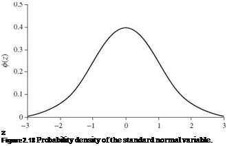
Подпись: z Figure 2.18 Probability density of the standard normal variable.

The integral result of Eq. (2.62) is not analytically available. A table of the standard normal CDF, such as Table 2.2 or similar, can be found in many statistics textbooks (Abramowitz and Stegun, 1972; Haan, 1977; Blank, 1980;

TABLE 2.2 Table of Standard Normal Probability, Ф( z) = P(Z < z)

z

0.00

0.01

0.02

0.03

0.04

0.05

0.06

0.07

0.08

0.09

0.0

0.5000

0.5040

0.5080

0.5120

0.5160

0.5199

0.5239

0.5279

0.5319

0.5359

0.1

0.5398

0.5438

0.5478

0.5517

0.5557

0.5596

0.5636

0.5675

0.5714

0.5753

0.2

0.5793

0.5832

0.5871

0.5910

0.5948

0.5987

0.6026

0.6064

0.6103

0.6141

0.3

0.6179

0.6217

0.6255

0.6293

0.6331

0.6368

0.6406

0.6443

0.6480

0.6517

0.4

0.6554

0.6591

0.6628

0.6664

0.6700

0.6736

0.6772

0.6808

0.6844

0.6879

0.5

0.6915

0.6950

0.6985

0.7019

0.7054

0.7088

0.7123

0.7157

0.7190

0.7224

0.6

0.7257

0.7291

0.7324

0.7357

0.7389

0.7422

0.7454

0.7486

0.7517

0.7549

0.7

0.7580

0.7611

0.7642

0.7673

0.7704

0.7734

0.7764

0.7794

0.7823

0.7852

0.8

0.7881

0.7910

0.7939

0.7967

0.7995

0.8023

0.8051

0.8078

0.8106

0.8133

0.9

0.8159

0.8186

0.8212

0.8238

0.8264

0.8289

0.8315

0.8340

0.8365

0.8389

1.0

0.8413

0.8438

0.8461

0.8485

0.8508

0.8531

0.8554

0.8577

0.8599

0.8621

1.1

0.8643

0.8665

0.8686

0.8708

0.8729

0.8749

0.8770

0.8790

0.8810

0.8830

1.2

0.8849

0.8869

0.8888

0.8907

0.8925

0.8944

0.8962

0.8980

0.8997

0.9015

1.3

0.9032

0.9049

0.9066

0.9082

0.9099

0.9115

0.9131

0.9147

0.9162

0.9177

1.4

0.9192

0.9207

0.9222

0.9236

0.9251

0.9265

0.9279

0.9292

0.9306

0.9319

1.5

0.9332

0.9345

0.9357

0.9370

0.9382

0.9394

0.9406

0.9418

0.9429

0.9441

1.6

0.9452

0.9463

0.9474

0.9484

0.9495

0.9505

0.9515

0.9525

0.9535

0.9545

1.7

0.9554

0.9564

0.9573

0.9582

0.9591

0.9599

0.9608

0.9616

0.9625

0.9633

1.8

0.9641

0.9649

0.9656

0.9664

0.9671

0.9678

0.9686

0.9693

0.9699

0.9706

1.9

0.9713

0.9719

0.9726

0.9732

0.9738

0.9744

0.9750

0.9756

0.9761

0.9767

2.0

0.9772

0.9778

0.9783

0.9788

0.9793

0.9798

0.9803

0.9808

0.9812

0.9817

2.1

0.9821

0.9826

0.9830

0.9834

0.9838

0.9842

0.9846

0.9850

0.9854

0.9857

2.2

0.9861

0.9864

0.9868

0.9871

0.9875

0.9878

0.9881

0.9884

0.9887

0.9890

2.3

0.9893

0.9896

0.9898

0.9901

0.9904

0.9906

0.9909

0.9911

0.9913

0.9916

2.4

0.9918

0.9920

0.9922

0.9925

0.9927

0.9929

0.9931

0.9932

0.9934

0.9936

2.5

0.9938

0.9940

0.9941

0.9943

0.9945

0.9946

0.9948

0.9949

0.9951

0.9952

2.6

0.9953

0.9955

0.9956

0.9957

0.9959

0.9960

0.9961

0.9962

0.9963

0.9964

2.7

0.9965

0.9966

0.9967

0.9968

0.9969

0.9970

0.9971

0.9972

0.9973

0.9974

2.8

0.9974

0.9975

0.9976

0.9977

0.9977

0.9978

0.9979

0.9979

0.9980

0.9981

2.9

0.9981

0.9982

0.9982

0.9983

0.9984

0.9984

0.9985

0.9985

0.9986

0.9986

3.0

0.9987

0.9987

0.9987

0.9988

0.9988

0.9989

0.9989

0.9989

0.9990

0.9990

3.1

0.9990

0.9991

0.9991

0.9991

0.9992

0.9992

0.9992

0.9992

0.9993

0.9993

3.2

0.9993

0.9993

0.9994

0.9994

0.9994

0.9994

0.9994

0.9995

0.9995

0.9995

3.3

0.9995

0.9995

0.9995

0.9996

0.9996

0.9996

0.9996

0.9996

0.9996

0.9997

3.4

0.9997

0.9997

0.9997

0.9997

0.9997

0.9997

0.9997

0.9997

0.9997

0.9998

NOTE: Ф(-г) = 1 – Ф(г), z > 0.

Devore, 1987). For numerical computation purposes, several highly accurate approximations are available for determining Ф(z). One such approximation is the polynomial approximation (Abramowitz and Stegun, 1972)

Ф(z) = 1 – ф(z)(b1t + b2t2 + b3t3 + b4t4 + b5t5) for z > 0 (2.63)

in which t = 1/(1 + 0.2316419z), b1 = 0.31938153, b2 = -0.356563782, b3 = 1.781477937, b4 = -1.821255978, and b5 = 1.33027443. The maximum absolute error of the approximation is 7.5 x 10⁻⁸, which is sufficiently accurate for most practical applications. Note that Eq. (2.63) is applicable to the non-negative­valued z. For z < 0, the value of standard normal CDF can be computed as ФЫ = 1 – Ф(|z|) by the symmetry of ф(z). Approximation equations, such as

Eq. (2.63), can be programmed easily for probability computations without needing the table of the standard normal CDF.

Some Continuous Univariate Probability Distributions Подпись: for 0.5 < p < 1 Подпись: (2.64)

Equally practical is the inverse operation of finding the standard normal quantile zp with the specified probability level p. The standard normal CDF table can be used, along with some mechanism of interpolation, to determine zp. However, for practical algebraic computations with a computer, the following rational approximation can be used (Abramowitz and Stegun, 1972):

in which p = ), t = y/-2 ln(1 – p), c0 = 2.515517, ci = 0.802853, c2 =

0.010328, d1 = 1.432788, d2 = 0.189269, and d3 = 0.001308. The correspond­ing maximum absolute error by this rational approximation is 4.5 x 10⁻⁴. Note that Eq. (2.64) is valid for the value of Ф^) that lies between [0.5, 1]. When p < 0.5, one can still use Eq. (2.64) by letting t = J-2 x ln(p) and attaching a negative sign to the computed quantile value. Vedder (1995) proposed a sim­ple approximation for computing the standard normal cumulative probabilities and standard normal quantiles.

Example 2.16 Referring to Example 2.14, determine the probability of more than five overtopping events over a 100-year period using a normal approximation.

Solution In this problem, the random variable X of interest is the number of over­topping events in a 100-year period. The exact distribution of X is binomial with parameters n = 100 and p = 0.02 or the Poisson distribution with a parameter v = 2. The exact probability of having more than five occurrences of overtopping in 100 years can be computed as

Подпись: P (X > 6) =Подпись:Подпись:Some Continuous Univariate Probability Distributions

Подпись: = 1 - P (X < Подпись: 100 x Подпись: (0.02)x (0.98)100-x Подпись: x = 6

P(X > 5) =

= 1 – 0.9845 = 0.0155

As can be seen, there are a total of six terms to be summed up on the right-hand side. Although the computation of probability by hand is within the realm of a reasonable task, the following approximation is viable. Using a normal probability approxima­tion, the mean and variance of X are

/Px = np = (100)(0.02) = 2.0 al = npq = (100)(0.02)(0.98) = 1.96

The preceding binomial probability can be approximated as

P(X > 6) ^ P(X > 5.5) = 1 – P(X < 5.5) = 1 – P [Z < (5.5 – 2.0)/УЇ96]

= 1 – Ф(2.5) = 1 – 0.9938 = 0.062

DeGroot (1975) showed that when np 1.5 >

1.07, the error of using the normal dis­tribution to approximate the binomial probability did not exceed 0.05. The error in the approximation gets smaller as the value of np15 becomes larger. For this exam­ple, np15 = 0.283 < 1.07, and the accuracy of approximation was not satisfactory as shown.

Example 2.17 (adopted from Mays and Tung, 1992) The annual maximum flood magnitude in a river has a normal distribution with a mean of 6000 ft3/s and standard deviation of 4000 ft3/s. (a) What is the annual probability that the flood magnitude would exceed 10,000 ft3/s? (b) Determine the flood magnitude with a return period of 100 years.

Solution (a) Let Q be the random annual maximum flood magnitude. Since Q has a nor­mal distribution with a mean xq = 6000 ft3/s and standard deviation oq = 4000 ft3/s, the probability of the annual maximum flood magnitude exceeding 10,000 ft3/s is

P(Q > 10, 000) = 1 – P [Z < (10, 000 – 6000)/4000]

= 1 – Ф(1.00) = 1 – 0.8413 = 0.1587

(b) A flood event with a 100-year return period represents the event the magnitude of which has, on average, an annual probability of 0.01 being exceeded. That is, P(Q > 7100) = 0.01, in which 7100 is the magnitude of the 100-year flood. This part of the problem is to determine 7100 from

P(Q < 7100) = 1 – P(Q > 7100) = 0.99

because P(Q < 7100) = P {Z < [(7100 – xq)/oq]}

= P [Z < (7100 – 6000)/4000]

= Ф[71.00 – 6000)/4000] = 0.99

From Table 2.2 or Eq. (2.64), one can find that Ф(2.33) = 0.99. Therefore,

(7100 – 6000)/4000 = 2.33

which gives that the magnitude of the 100-year flood event as 7100 = 15, 320 ft3/s.

Poisson distribution

The Poisson distribution has the PMF as

e — vV x

px(x | v) =—;— for x = 0,1,2,… (2.53)

x!

where the parameter v > 0 represents the mean of a Poisson random variable. Unlike the binomial random variables, Poisson random variables have no upper bound. A recursive formula for calculating the Poisson PMF is (Drane et al., 1993)

Px (x | v) = (X) Px (x — 11 v) = Rp (x) Px (x — 11 v) for x = 1,2,… (2.54)

with px(x = 0 | v) = e—v and RP (x) = v/x. When v and p ^ 0 while np = v = constant, the term RB (x) in Eq. (2.52) for the binomial distribution becomes RP (x) for the Poisson distribution. Tietjen (1994) presents a simple recursive scheme for computing the Poisson cumulative probability.

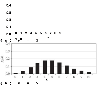
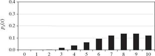
For a Poisson random variable, the mean and the variance are identical to v. Plots of Poisson PMFs corresponding to different values of v are shown in Fig. 2.17. As shown in Fig. 2.15, Poisson random variables also have the same re­productive property as binomial random variables. That is, the sum of several independent Poisson random variables, each with a parameter vk, is still a Poisson random variable with a parameter v1 + v2 + ■ ■ ■ + vK. The skewness

Poisson distribution

Poisson distribution

x

(c) v = 9

Figure 2.17 Probability mass functions of Poisson random variables with different parameter values.


Poisson distribution

coefficient of a Poisson random variable is 1Д/ЇЇ, indicating that the shape of the distribution approaches symmetry as v gets large.

The Poisson distribution has been applied widely in modeling the number of occurrences of a random event within a specified time or space interval. Equation (2.2) can be modified as

p-lt ( W )X

Px (x | X, t) = for x = 0,1,2,… (2.55)

X!

in which the parameter X can be interpreted as the average rate of occurrence of the random event in a time interval (0, t).

Example 2.15 Referring to Example 2.14, the use of binomial distribution assumes, implicitly, that the overtopping occurs, at most, once each year. The probability is zero for having more than two overtopping events annually. Relax this assumption and use the Poisson distribution to reevaluate the probability of overtopping during a 100-year period.

Solution Using the Poisson distribution, one has to determine the average number of overtopping events in a period of 100 years. For a 50-year event, the average rate of overtopping is X = 0.02/year. Therefore, the average number of overtopping events in a period of 100 years can be obtained as v = (0.02)( 100) = 2 overtoppings. The probability of overtopping in an 100-year period, using a Poisson distribution, is

P (overtopping occurs in a 100-year period)

= P (overtopping occurs at least once in a 100-year period)

= 1 — P (no overtopping occurs in a 100-year period)

= 1 — p(X = 0 | v = 2) = 1 — e—2 = 1 — 0.1353 = 0.8647

Comparing with the result from Example 2.14, use of the Poisson distribution results in a slightly smaller risk of overtopping.

To relax the restriction of equality of the mean and variance for the Pois­son distribution, Consul and Jain (1973) introduced the generalized Poisson distribution (GPD) having two parameters в and X with the probability mass function as

в(в I xX)n 1e (e +xX)

px(x | в, X) = for x = 0,1,2,…; X > 0 (2.56)

x!

The parameters (в, X) can be determined by the first two moments (Consul, 1989) as

вв

E(X)=1—X Var(X)=(T-D3 e.57)

The variance of the GPD model can be greater than, equal to, or less than the mean depending on whether the second parameter X is positive, zero, or negative. The values of the mean and variance of a GPD random variable tend to increase as в increases. The GPD model has greater flexibility to fit various types of random counting processes, such as binomial, negative binomial, or Poisson, and many other observed data.

Wafer Quality Specialist

If a site lacks water, it is important to deter­
mine the cost of obtaining it. If the site is served by the local municipality, the water company may be able to give you an estimate. If the site is rocky, you may need to excavate trenches by blasting the surrounding rock. If you must drill a well, the neighbors or the local well driller can inform you of the depth of surrounding wells and give you information about water quality. If the site already contains a well, ensure that the submersible pump was manufactured after 1979, or that it is safe. If the

Подпись: у

The American Society of Dowsers Inc., dowsers. org

BioGeometry, biogeometry. com and vesica. org The British Society of Dowsers, geomancy. org The Canadian Society of Dowsers, canadiandowsers. org

The Canadian Society of Questers, questers. ca International Institute for Bau-Biology & Ecology, buildingbiology. net

Pyramid School of Feng Shui, Nancilee Wydra, fengshuibydesignonline. com

a. Information provided by Dulwich Health and available at dulwichhealth. co. uk.

b. Alf Riggs. "Harmful Effects from Earth Radia­tion & Electrical Fields" [online]. [Cited Decem­ber 19,2007.] whale. to/v/riggsi. html

c. Hans Nieper."Modern Medical CancerTherapy Following the Decline of Toxic Chemotherapy." Townsend Letter for Doctors & Patients. Novem­ber 1996, pp. 88-89. Dr. Nieper’s Revolution in Technology, Medicine and Society. MIT Verlag, 1985, pp. 206,222. Lecture notes from a medical seminar in Los Angeles, July 4,1986, pp. 13-15, 22, 28, available from Brewer Science Library, mwt. net/~drbrewer/other. htm. See also Hans

A. Nieper et al. The Curious Man: The Life and Works of Dr. Hans Nieper. Avery, 1998.

d. Kathe Bachler. "Noxious Earth Energies and Their Influence on Human Beings" [online]. [Cited December 19,2007.] whale. to/v/bachler. html. See also Kathe Bachler. Discoveries of a Dowser. 5th ed., Veritas, 1984 and Kathe Bachler. Earth Radiation. Wordmasters, 1989.

e. AlfRiggs."MyalgicEncephalomyelitis"[online]. [Cited Decembers,2007.] alfredriggs. com

J. David McAuley has practiced architecture in Canada for 29 years using Building Biology, feng shui, and Earth energy dowsing. He is currently studying BioGeometry. David designs buildings to support health in balance with the environment, including sacred spaces, healing retreat centers, and socially conscious spaces for those in need. He can be contacted at 519-823-2441 or jdm-arch .com.

oils in older pumps contain PCBs, they repre­sent a serious health threat should a rupture occur. Whatever the source of potable water, it should be tested by a professional and filtered or purified as required. Water quality will be discussed further in Division n.

HIGH-OCCUPANCY VEHICLE LANES

Another method that is being increasingly used to relieve congestion on urban free­ways is the establishment of high-occupancy vehicle (HOV) lanes. Although the first instances of use in California in the early 1970s met with much public resistance, the idea was revisited and accepted more readily during the mid-1980s and continues to grow in acceptance in highly congested urban traffic areas (Ref. 9). The concept is to provide a separate lane or lanes for high-occupancy vehicles such as buses, carpools, vanpools, and other ride-sharing modes of transportation. This, in turn, provides a positive incentive for the general public to seek out ride-sharing transportation modes, both public and private. The overall goal is to move more people in fewer vehicles.

2.13.1 Planning Considerations

The following transportation system goals can be achieved by proper development and use of HOV lanes (Ref. 3):

• To maximize the person-moving capacity of roadway facilities by providing improved level of service for high-occupancy vehicles, both public and private

• To conserve fuel and to minimize consumption of other resources needed for transportation

• To improve air quality

• To increase overall accessibility while reducing vehicular congestion

Designing and implementing HOV lanes should be limited to those cases where extreme congestion occurs on a regular basis. They should be used in conjunction with other programs that will promote the use of ride-sharing modes, such as park- and-ride lots, park-and-pool lots, and information services to facilitate bus and ride – share needs.

The following guidelines should be used to determine when an HOV lane should be implemented:

• Compatibility with other plans

HOV lanes should be part of an overall transportation plan.

Community support should be obtained for developing HOV lanes.

Intense, recurring congestion should be occurring on the freeway general-purpose lanes.

Peak-period traffic per lane should be approaching capacity (1700 to 2000 vehicles per hour).

During peak periods, average speeds on the freeway main lanes during nonincident conditions should be less than 30 mi/h (48 km/h) over a distance of about 5 mi (8 km) or more.

Compared with using the freeway general-purpose lanes, the HOV lanes should offer a travel time savings of at least 5 to 7 min during the peak hour.

• Coordination with travel patterns that encourage ridesharing

Significant volume of peak-period trips (e. g., more than 6000 home-based work trips during the peak hour) on the freeway should be destined to major activity centers or employment areas in or along the freeway corridor.

At least 65 to 75 percent of peak-period freeway trips to major activity centers should be 5 mi (8 km) or more in length.

Resulting ride-share demand should be sufficient to generate HOV volumes that are high enough to make the facility appear to be adequately utilized; volumes may vary by type and location of facility.

• A design that allows for safe, efficient, and enforceable operation

Habitat Builds Barrier-Free Homes

Habitat Builds Barrier-Free Homes

SIMPLE, SINGLE-STORY HOUSES are

not only inexpensive to build but also lend themselves well to barrier-free (handicap-аccessible) eonstruction.

In addition to the obvious differences that relate to wheelchair accessibility—

4

wider hallways and doorways, a ramp instead of a stairway at the entrvwav—

/ 4 4

many other smaller details help make these homes easier for their owners to use and enjoy.

The key to building or retrofitting a house for wheelchair accessibility is recognizing the modified reach of a seated person. You can start by raising the position of electrical outlets and
lowering the height of light switches, closet poles, shelves, and countertops. These easily made alterations help make day-to-day life more convenient for someone in a wheelchair.

Bathrooms and kitchens require special attention. Plenty of strategically placed grab bars are important; place them around the toilet and in and around the tub/shower. Extra space in the bathroom—so a wheelchair can get in and maneuver around—is essential, too. In the kitchen, lowered stovetop, sink, and cabinets help make it possi­ble for someone in a wheelchair to prepare and serve meals and clean up.

Recognizing the increasing need for barrier-free housing, the Knox­ville, Tennessee, Habitat affiliate spon­sored a contest to design an adapt­able, inexpensive, barrier-free house. Two designs were selected as winners; both are available to any affiliate through Habitat for Humanity Inter-

О 4

national. With the leading edge of the baby-boom population already past 55, and modern medicine keeping us alive ever longer, more and more of us may come to appreciate housing that’s flexible enough to adapt to our needs as the years go by.

-Vincent Laurence

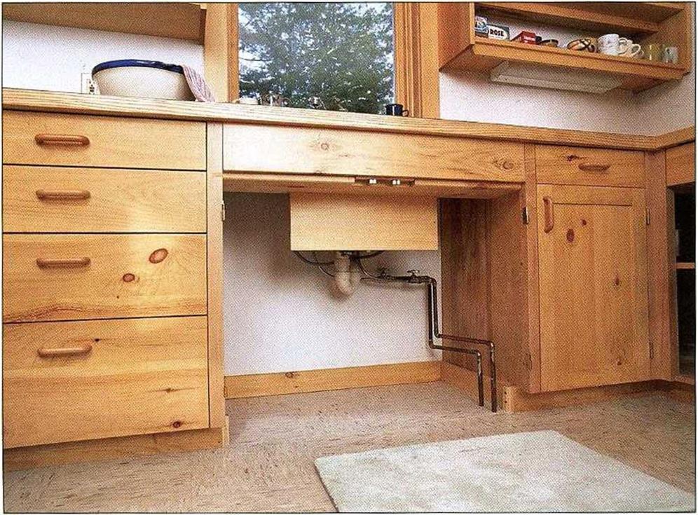
MODIFY CABINETS FOR WHEELCHAIR ACCESS.

Lower countertops and desk-type openings can make the kitchen much more accessible.

[Photo by Steve Culpepper, courtesy of Fine Homebuilding magazine The Taunton Press, Inc.|

Techniques FRAMING HEADOUTS

Habitat Builds Barrier-Free HomesHabitat Builds Barrier-Free Homes

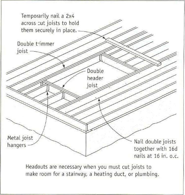
SOMETIMES JOISTS MUST be cut to allow room for a stairway, a heater vent in the floor, or a tub trap in the bathroom. Such an opening is called a headout. As shown in the illustration at right, regular 2x joists (not I-joists) can be cut and supported by a header joist that is fas­tened to parallel joists. If the opening is larger than 4 ft., double both the side and the header joists. Attach the doubles with 16d nails spaced 16 in. o. c.

A common mistake made by carpenters framing a headout is not taking into account the thickness of the header joists. Remember to factor in these joists when determining the size of your floor opening. If, for example, you need a 2-ft.-Long floor opening, cut the joists at 2 ft. 3 in. to leave room for the single-header joist at each end. For double-header joists, cut the joists at 2 ft. 6 in.

Подпись: NAIL OFF 2x JOISTS. To install 2x joists, drive a pair of 16d nails through the rim joist into the end of the joist. Then drive a toenail through each side of the joist into the sill.

Roll and nail the joists

Once the joists arc cut to length and in posi­tion, carpenters say that it’s time to “roll” them. This just means setting the joists on edge, aligning them with their layout, and nailing them in place. If you are working with 2x joists, it’s important to sight down each joist to see whether there’s a how or a crown, and then set the joist with the crown facing up.

Drive two 16d nails through the rim joist directly into the end of the joist—one nail near the top and one near the bottom (see the photo at right). Most codes also require that joists be toenailed (one 16d on each side) to the sill plates and supporting girders. To nail off an 1-joist, drive a 16d nail through the rim joist and into each chord, then nail the chord to the sill on both sides of the web.

Подпись: Г IПодпись: Helping HandПодпись: Make blocking from bad joists. When using 2x lumber for joists, avoid boards that are bowed or twisted or have large knots. Set them aside, then cut them up for blocking.Make sure that all the joists are nailec. securely. This is important for safety reasons, for quality workmanship, and for meeting the building inspection. Once all the joists are nailed upright, stop and check for symmetry— make sure the line of one joist is parallel with another. This is an easy way to spot layout mistakes. Take the time to check the framing against the details shown on the plans. Cor­rections are much easier to make now than after the floor sheathing is installed. Enjoy the moment. Joists on edge are beautiful in their own right, clearly and unmistakably showing the promise of a new building.
STEP7 Install Extra Joists and Blocking

Until recently, extra joists were often required under walls that ran parallel to the joists, because they helped support the roof struc­ture. Most houses built these davs use roof

і

trusses, however, which are engineered to span from outside wall to outside wall without the need for interior support. There usually isn’t a need to install extra joists under walls, though some local codes still require them. Check with your town or city building department to make sure.

Similarly, wood or metal bridging is no longer required. Installed in crossed pairs between joists, bridging is often visible

SHINGLE REPAIRS

To remove wood shingles, use scrap blocks to ele­vate the butt ends of the course above. Work the blade of a chisel into the butt end of the defective shingle, and with twists of your wrist, split the shingle into slivers. Before fitting in a new shin­gle, remove the nails that held the old one. Slide a hacksaw blade or, better, a shingle ripper (also known as a slate hook) up under the course above and cut through the nail shanks as far down as possible. If you use a hacksaw blade, wear a heavy glove to protect your hand.

Wood shingles should have a!4-in. gap on both sides, so size the replacement shingle lA in. narrower than the width of the opening. Tap in the replacement with a wood block. If the replacement shingle won’t slide in all the way, pull it out and whittle down its tapered end, using a utility knife. It’s best to have nail heads covered by the course above, but if that’s not pos­sible, place a dab of urethane caulk beneath each nail head before hammering it down. Use two 4d galvanized shingle nails per shingle, each set in 14 in. from the edge.

image176

GOT

Moss-covered shingles and shakes are common in moist, shaded areas. Hand scrape or use a wire brush to take the moss off. Keep it off by stapling 10-gauge or 12-gauge copper wire to a course of shingle butts all the way across the roof. Run one wire along the ridge and another halfway down. During rains, a dilute copper solution will wash down the shingles, discourag­ing moss. A nice alternative to toxic chemical treatments.

A Medley of Roofing Types

Although this section contains a few modest repairs a novice can make, most of the roof types discussed here should be installed by a roofing specialist. You’ll also find suggestions for deter­mining the quality of an installation as well as a few inspired tips.

FLAT ROOFS

Actually, no roof should be completely flat, or it won’t shed water. But flat roof is a convenient term for a class of multimembrane systems. At one time, builtup roofs (BURs) once represented half of all flat roof coverings. BURs consisted of alternative layers of heavy building paper and hot tar. Today, modified bitumin (MB) is king, with cap membranes torched-on to fuse them to fiber­glass-reinforced interplies or base coats. MB sys­tems are durable and adhere well to dissimilar materials and difficult joints, but an inexpert torch user can damage the membranes and set a house on fire. For that reason, future roofs are likely to employ hot-air welding, cold-press adhesives, and roll membranes with self-sticking edges.

Causes of flat-roof failure. Whatever the mate­rials used, flat roofs are vulnerable because water pools on them, people walk on them, and the sun degrades them unless they’re properly maintained. Here are the primary causes of membrane damage:

► Water trapped between layers, because of improper installation. This is caused by installing roofing too soon after rain or when the deck was moist with dew. The trapped water expands, resulting in a blister in the membrane. In time, the blister is likely to split.

► Inadequate flashing around pipes, skylights, and adjoining walls.

► Drying out and cracking from UV rays— usually after the reflective gravel covering has been disturbed.

► People walking on the roof, or roof decks placed directly on a flat roof membrane. Roof decks should be supported by "floating posts" bolted through the sheathing to rafters and correctly flashed.

Repairing roof blisters. If there are no leaks below and the blister is intact, stay away from it! Don’t step on it, cut it, or nail through it. How­ever, if it has split, press it to see what comes out. If the roof is dry, only air will escape; if the roof is wet, water will emerge. In the latter case, let the inside of the blister dry by holding the side open with wood shims; if you’re in a hurry, use a hair dryer. Once the blister has dried inside, patch it.

LAYING A FLAT ROOF

image177

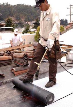
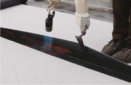
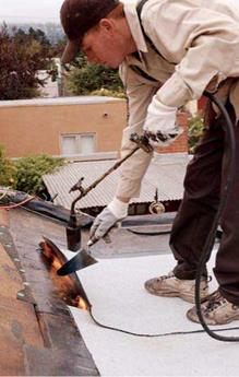
In the final phase of a MB roof, an installer torch-welds a granular surface membrane to an interply sheet or directly to a base sheet. The granular surface is somewhat more expensive at installation, but it is cost-effective in the long run because it doesn’t need periodic recoating.


image178

Once the granular membrane is down, its overlapping edges are often lifted and torched again to ensure sound adhesion and a waterproof seam.


image180

The intersection of flat and sloping roof sections is worth extra attention. Run MB membranes at least 10 in. (vertical height) up the sloping section. Then overlap those membranes with the underlayment materials and asphalt shingles.


image179

Roofers refer to the molten material being forced out by the pressure of the trowel as wet seams—the mark of a successful installation.


Подпись: Ilie-ROOT UNDERLAYMENT A rubberized asphalt underlayment reinforced with fiberglass, layfastSBS®, is getting a lot of buzz among professionals. Specified for tile roofs, it's installed in two layers (double-papered) with 36.-in.-wide sheets overlapped by 19 in. Tiles often gouge building paper underlayment during installation, but not this stuff, which is also specified for shake, shingle, and metal roofs.

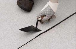
Professionals repair split blisters with a three – course patch, which requires no nails.

1. Trowel on a J4-in.-thick layer of an elas­tomeric mastic, such as Henry 208 Wet Patch®, carefully working it into both sides of the split. Extend the mastic at least 2 in. beyond the split in all directions.

2. Cut a piece of "yellow jacket” (yellow fiberglass roofer’s webbing) slightly longer than the split and press it into the mastic; this reinforces the patch.

3. Apply another!4-in. layer of mastic over the webbing, feathering its edges so it can shed water.

A three-course patch is also effective on failed flashing, where dissimilar materials meet, and for other leak-prone areas.

SITE PLANNING

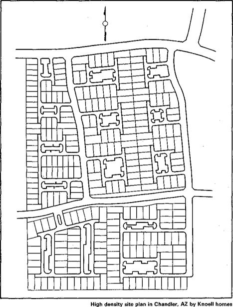
Successful approaches to affordable housing require more efficient utilization of land than has often characterized American home building practices in the past.

In most of the demonstration projects, reducing land cost per housing unit was the biggest single factor in achieving affordability. Lower housing cost is therefore closely linked to greater density of land utilization per acre.

This, in turn, poses challenges in the design and aesthetics of housing and land use to maintain and even improve liveability in the context of increased density.

Following are guidelines for site planning:

• Encourage plans to increase density and maintain open space.

• Avoid development plans with wide streets in grid patterns, large lots, deep setbacks, and low density.

• Encourage open space and preservation of natural features in site plans.

• Support cluster plans which increase density and create open space, provide adequate parking, and design privacy landscaping.

• Reduce or eliminate setbacks from all four lot boundaries.

• Support "zero-lot-line" and "Z" lot configurations.

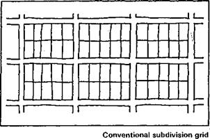
Подпись: Traditional ApproachesSITE PLANNINGTraditional housing development plans prevalent in the Post-World War II oeriod are characterized by a grid oattern of wide streets with houses on ‘arge lots with large setbacks.

Such plans were widely viewed as affording privacy and providing desirable residential environments. These views were reflected in local housing ordinances, which often restricted density per acre and specified large setbacks.

However, there is little reason to believe that this extravagant use of land made any meaningful contribution

to the goals of desirability and privacy. There is nothing intrinsic in the arrangement which promotes or increases privacy, and "desirable residential environments" often turned out to be urban sprawl. In many instances, little provision was made fon open or common land or for integration of common open space in the overall design of the development.

This type of development does not make efficient use of community seryices such as roads, and water and sewer systems because of the rela­tively low density. The cost of their wasted capacity is borne by both residents and the public sector.

Подпись: Innovative ApproachesThere are a number of ways in which well-planned higher density can contribute to, rather than detract from, beauty and liveability. For example, a greater amount of common open space and more possibilities for preservation of attractive natural features of the site are often easier rather than more difficult to incor­porate into good plans for higher – density occupancy.
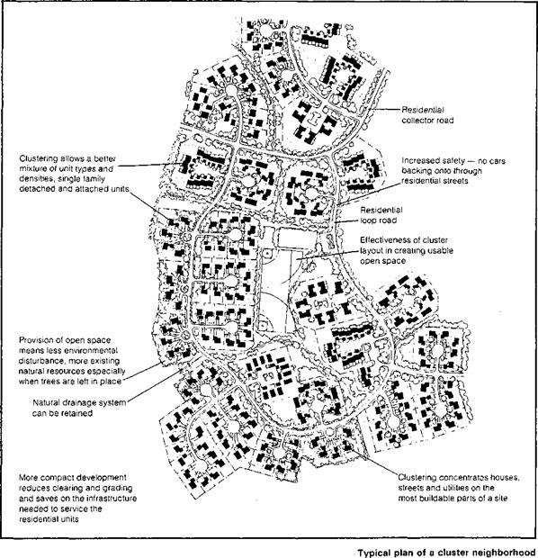
Other potential problems of higher density can be overcome through innovative planning. Two such problems are privacy and parking. Privacy can be provided by coordi­nating arrangements of fences and/or planting. For attached units, sound conditioning can be incorporated into common walls.

SITE PLANNING

Rear yards and front entry courts can be enclosed. Parking can be provided through placement of garages or carports within parking areas and by use of planted islands.


SITE PLANNING

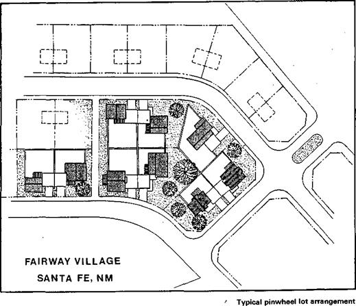
Подпись: ClusteringMany clustering arrangements have been successfully designed to combine higher density, beauty, and liveability. Clusters can be incorporated into site development plans to preserve open space for community use while reducing development costs.

In addition, it has been found that such arrangements can increase the sense of community among residents within each cluster and among adjacent and neighboring clusters. A cluster can become a psychologically identifiable "place" more easily than can rows of detached houses on rectangular lots. Groups of clusters can relate to each other through joint access to common land.

SITE PLANNING
Clusters can be designed for siting single-family detached or attached homes, duplexes, quadplexes, etc.

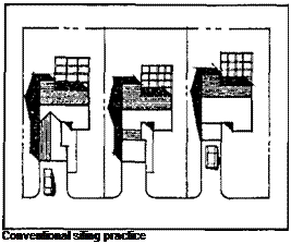
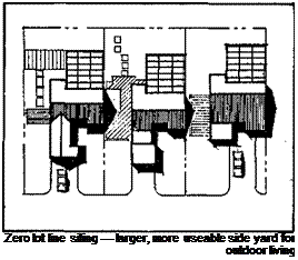
Подпись: Reduction or Elimination of Setback RequirementsПодпись:Подпись: Zero lot line siting — larger, more useable side yard for outdoor living The traditional practice of using large setbacks from all four boundaries of the lot reduces the usability of land on both sides of the house, particu­larly on smaller lots. By placing the house directly on the lot line on one side, usable land on the other side is doubled.
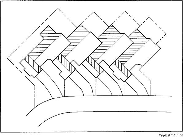
This "zero-lot-line" approach is basically a detached version of the duplex home. That is, by moving one duplex unit away from the common wall to the other side of the lot, high density is maintained while creating a freestanding single-family detached subdivision. This approach combines two small unusable side yards into one large usable side yard. Usually, main living areas are oriented toward the side, taking advantage of the "court."

On the smaller lots that most often are used in affordable housing developments, this can make the difference between having or not having usable outdoor space.

SITE PLANNING

Подпись: “Z” Lot ConfigurationAn adaptation of the zero-lot-line approach is an innovative concept called "Z" lots. Sometimes called "herringbone" or "sawtooth", these angled lots expand frontages and expose more of the home to the street. Because of the angle, garages don’t dominate the streetscape as much as in more traditional rectan­gular lot layouts, especially if garage door locations are alternated. The JVAH site in Everett, WA, included a variation on the "Z" lot approach with garages set at an angle with the homes and the street. ‘

Permeability Tests of Saturated Soils and Aggregates

Traditionally in geotechnical engineering, the saturated permeability is estimated in the laboratory in a constant head test for coarse grained soils whereas a falling head test is used for fine grained soils. An oedometer test can also provide a measure of the saturated permeability for fine grained soils in the laboratory. Field tests which provide a measure of the saturated permeability are usually a kind of pumping well test, or injection test.

3.3.1.1 Constant Head Permeability Test

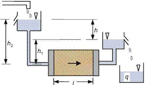
A constant head permeability test is usually used for coarse grained soils. The sam­ple is placed in the permeameter where a constant head drop is applied to the sample and the resulting seepage quantity is measured (see Fig. 3.5).

Подпись: Fig. 3.5 Constant head permeability test Permeability Tests of Saturated Soils and Aggregates

By rearranging and substituting into Eq. 2.15, the permeability K is given as:

where q is the discharge (L3/T), L is the specimen length (L), A is the cross section area of the specimen (L2) and h is the constant head difference (L).

There are limitations to the use of a permeameter test for pavement materials. Sub-bases or drainage layers normally contain particles with a maximum nominal size between about 20 and 80 mm. It has been suggested that to obtain reliable per­meability measurements that the value of the ratio of the permeameter diameter to the maximum particle diameter should be between 8 and 12. However, standard permeameters are generally too small and too fragile to allow the largest particles to be included and to achieve correct compaction. Head (1982) describes a 406 mm diameter permeability cell suitable for gravel containing particles up to 75 mm.

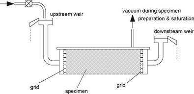
To help overcome this limitation, the UK Department of Transport (1990) intro­duced a large, purpose-designed, permeameter for testing road construction aggre­gates (Fig. 3.6). It measures horizontal permeability at low hydraulic gradients as these are the hydraulic conditions that might be anticipated in granular pavement layers.

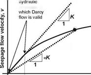
Normally, Darcy flow is assumed to be the regime of permeating water in the soil or aggregate layers under a road, i. e. the water percolates at sub-critical velocities and without eddy-flow when moving from small to large pore spaces. This means that energy losses are only due to friction between the water and the surrounding solids and that a constant value of coefficient of permeability, K, can be defined. When coarse materials, with large pores, are tested for permeability in equipment such as that illustrated in Fig. 3.6, care must be taken to ensure that Darcy conditions are maintained throughout the test. Under many conventional test conditions, high hydraulic gradients are applied (much larger than in-situ) in order to obtain results in a convenient time scale. If such hydraulic gradients are applied to materials with large pores, eddy flows may develop in the large pores and more energy will be lost than Darcy conditions would predict. If the user is unaware of these conditions, the value of coefficient of permeability, K, will be under-estimated (see Fig. 3.7).

water supply

Permeability Tests of Saturated Soils and Aggregates

Ra"ge, of Darcy flow.

Подпись:Подпись: Hydraulic gradient, iPermeability Tests of Saturated Soils and Aggregatesgradients in Constant 9radient

Measured A response

Wrong interpretation of data point A using Darcy assumptions, leading to an underestimation of K

For this reason, tests should be performed at variable hydraulic gradients on coarse materials. Hydraulic gradients less than 0.1 may be required to achieve Darcy con­ditions. Alternatively, more advanced permeability formulations may be used such as those given in Eq. 2.21.

Binomial distribution

The binomial distribution is applicable to random processes with only two types of outcomes. The state of components or subsystems in many hydrosystems can be classified as either functioning or failed, which is a typical example of a binary outcome. Consider an experiment involving a total of n independent trials with each trial having two possible outcomes, say, success or failure. In each trial, if the probability of having a successful outcome is p, the probability of having x successes in n trials can be computed as

Px(x) = Cn, xpxqn-x for x = 0,1,2,…,n (2.51)

where Cn, x is the binomial coefficient, and q = 1 – p, the probability of having a failure in each trial. Computationally, it is convenient to use the following recursive formula for evaluating the binomial PMF (Drane et al., 1993):

Px(x | n, p) = (——————- x——– JVqjPx(x — 11 n, p) = Rb(x)Px(x — 11 n, p) (2.52)

for x = 0, 1,2,…, n, with the initial probability px(x = 0|n, p) = qn. A simple recursive scheme for computing the binomial cumulative probability is given by Tietjen (1994).

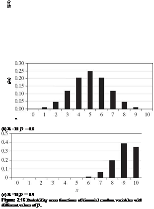
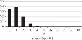
A random variable X having a binomial distribution with parameters n and p has the expectation E (X) = np and variance Var(X) = npq. Shape of the PMF of a binomial random variable depends on the values of p and q. The skewness coefficient of a binomial random variable is (q — p)/^/npq. Hence the PMF is positively skewed if p <q, symmetric if p = q = 0.5, and negatively skewed if p > q. Plots of binomial PMFs for different values of p with a fixed n are shown in Fig. 2.16. Referring to Fig. 2.15, the sum of several independent binomial random variables, each with a common parameter p and different nk s, is still a binomial random variable with parameters p and £knk.

Example 2.14 A roadway-crossing structure, such as a bridge or a box or pipe cul­vert, is designed to pass a flood with a return period of 50 years. In other words, the annual probability that the roadway-crossing structure would be overtopped is a 1-in-50 chance or 1/50 = 0.02. What is the probability that the structure would be overtopped over an expected service life of 100 years?

Solution In this example, the random variable X is the number of times the roadway­crossing structure will be overtopped over a 100-year period. One can treat each year as an independent trial from which the roadway structure could be overtopped or not overtopped. Since the outcome of each “trial” is binary, the binomial distribution is applicable.

Binomial distribution

Binomial distribution

Binomial distribution

The event of interest is the overtopping of the roadway structure. The probability of such an event occurring in each trial (namely, each year), is 0.02. A period of 100 years represents 100 trials. Hence, in the binomial distribution model, the parameters are p = 0.02 and n = 100. The probability that overtopping occurs in a period of 100 years can be calculated, according to Eq. (2.51), as

P (overtopping occurs in an 100-year period)

= P (overtopping occurs at least once in an 100-year period)

= P(X > 11 n = 100, p = 0.02)

100 100

= X) Px(x) = X) C1°°>x(0.02)x(0.98)100-x

x = 1 x = 1

This equation for computing the overtopping probability requires evaluations of 100 binomial terms, which could be very cumbersome. In this case, one could solve the problem by looking at the other side of the coin, i. e., the nonoccurrence of overtopping events. In other words,

P (overtopping occurs in a 100-year period)

= P (overtopping occurs at least once in a 100-year period)

= 1 — P (no overtopping occurs in a 100-year period)

= 1 — p( X = 0) = 1 — (0.98)100

= 1 — 0.1326 = 0.8674

Calculation of the overtopping risk, as illustrated in this example, is made under an implicit assumption that the occurrence of floods is a stationary process. In other words, the flood-producing random mechanism for the watershed under considera­tion does not change with time. For a watershed undergoing changes in hydrologic characteristics, one should be cautious about the estimated risk.

The preceding example illustrates the basic application of the binomial dis­tribution to reliability analysis. A commonly used alternative is the Poisson distribution described in the next section. More detailed descriptions of these two distributions in time-dependent reliability analysis of hydrosystems infras­tructural engineering are given in Sec. 4.7.

The Nilometers

One can readily see that in Egypt, measurement of the flood level has great importance. The management of the irrigation system is based on such measurements, as are the taxes, since the agricultural yield can be deduced almost automatically from the flood level. The level is quantified using graduated scales carved into stone; Strabo calls these [87] [88]

The Nilometers

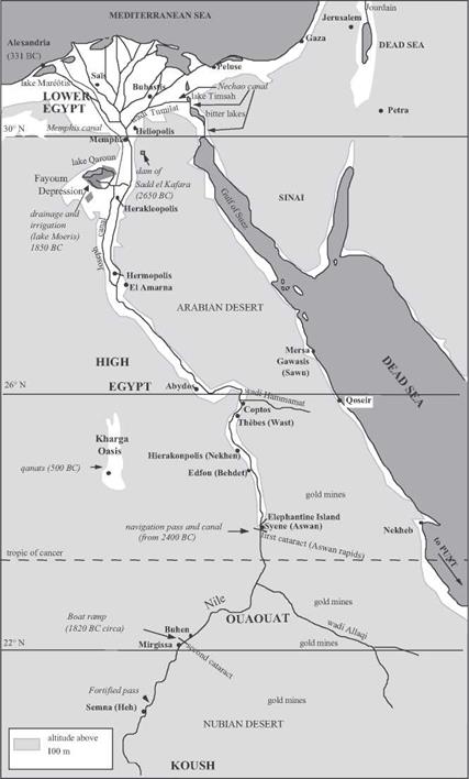
Figure 3.1 Major hydraulic works in ancient Egypt and Nubia.

scales “nilometers”. The most well-known nilometers[89] are those at the fortified pass of Semma, upstream of the second cataract (around 1800 BC), on Elephantine Island at Aswan, downstream of the first cataract (1800 BC), at the temple of Karnak at Thebes (800 BC), and near Memphis upstream of the delta (Figure 3.1). But much older nilome­ters surely existed, since flood levels were reported in the annals of the IVth and Vth dynasties (2500 – 2000 BC).[90] The unit of measurement is the nilometric cubit, or 0.525 m. The zero, or datum, of the nilometric scales is quite probably set at the low-flow level of the river, a level that can vary over time as the width of the river varies (a scale change occurred about 2000 BC). The scales have marks that correspond to favorable flood lev­els: a little more than 21 cubits at Elephantine, 12 to 14 cubits at Memphis, 7 cubits in the delta.

There are two particularly important locations for flood measurement: at

Elephantine (Aswan), the point of entry of the flood into Egypt proper, and at Memphis,

The Nilometers

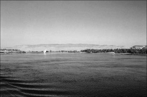
Figure 3.2 The Nile between Thebes and Aswan (photo by the author). One can see the contrast between the green irrigated plain (dark in the photo) and the arid hills in the background.

sentinel of the flood that will appear on the delta. In fact there are two nilometers at Aswan. According to tradition, a precise water level at Aswan is obtained in a well con­nected to the river, to dampen fluctuations caused by waves in the river itself. The date

of this concept is unknown. Let’s again listen to Strabo:

“The nilometer is a well, built of stone quarried from the banks of the Nile itself, in which there are marks indicating the greatest floods of the Nile, the smallest, and the average, for the water level in the wells rises and falls with that of the river. This is why there are marks on the walls of the wells, showing the peak flood levels and other levels. Inspectors examine the wells and communicate their observations to the rest of the population, for their informa­tion; they know well in advance, from these indications and their times, when the future inun­dation will occur, and can announce these forecasts. This information is useful not only to the farmers for the regulation of water distribution, for the dikes, the canals, and things of this nature, but also to the prefects for the estimation of public revenue, for these revenues increase with the strength of the flood.”[91]

According to Daniele Bonneau, the measurements begin at the end of June, at the summer solstice, and continue through the period of inundation to the end of October, and are made known throughout the valley for general public use.

Of course the Nile is also the prin­cipal “highway” of the country. The paintings of boats of the Nile found on protohistorical pottery are among the first such known depictions. Each city, each temple, has its fluvial port, generally constructed in the form of a “T”, with a basin connected to the Nile by a short canal.