Evaluation of the probability of multivariate normal random variables involves multidimensional integration as
Accurate evaluation for Ф(г |Rx) is generally difficult and often is resolved by approximations.
Bivariate normal probability. For abivariate case, Fortran computer programs for computing the lower left volume under the density surface, that is, Ф(а, b | p) = P(Z1 < a, Z2 < b | p), have been developed by Donnelly (1973) and Baughman (1988). The double integral for evaluating the bivariate normal probability can be reduced to a single integral as shown in Eq. (2.111). Several approximations have been derived (Johnson and Kotz, 1976). Derivation of bounds for the bivariate normal probability is presented in Sec. 2.7.3. For a bivariate normal probability, exact solutions have been obtained in the form of figures such as Fig. 2.28 for computing the upper-right volume under the bivariate standard normal density surface, that is, L(a, b | p) = P (Z1 > a, Z2 > b | p), in which L(a, b | p) can be expressed in terms of L(a, 0 | p) as
0, if (ab > 0 or ab = 0) and a + b > 0
1,  otherwise 2
|
P
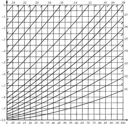
L(a, 0lp) for 0 < a < 1 and -1 < p < 0.
Values for a < 0 can be obtained using L(a, 01—p) = 0.5 – L(-a, 0lp)
Figure 2.28 Bivariate normal cumulative distribution function. (After Abramowitz and Stegun, 1972.)
|
The relationship between Ф^, b | p) and L(a, b | p) is
Ф(a, b | p) = —1 + Ф^) + Ф(Ь) + L(a, b | p) (2.118)
From the definitions of Ф^, b | p) and L(a, b | p) and the symmetry of the bivariate normal PDF, the following relations are in order:
Ф^, to| p) = Ф^) Ф(то, b | p) = Ф(Ь) (2.119a)
L(a, – to | p) = 1 – Ф^) L(-to, b | p) = 1 – Ф(Ь) (2.119b)
|
P
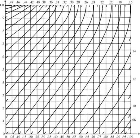
L(a, 0lp) for 0 < a < 1 and 0 < p < 1.
Values for a < 0 can be obtained using L(a, 01—p) = 0.5 – L(-a, 0lp) Figure 2.28 (Continued)
|
L(a, b | p) = L(b, a | p) (2.119c)
L(-a, b | p) + L(a, b | —p) = 1 – Ф(Ь) (2.119d)
L(-h, —k | p) — L(k, h | p) = 1 — Ф(К) — Ф(к) (2.119e)
Example 2.21 Consider two correlated normal random variables X1 and X2 with
their statistical properties being
E(X1) = 10 Var(X1) = 9 E(X2) = 5 Var(X2) = 4 Cov(Xb X2) = 3.6
Compute P(X1 < 13, X2 < 3).

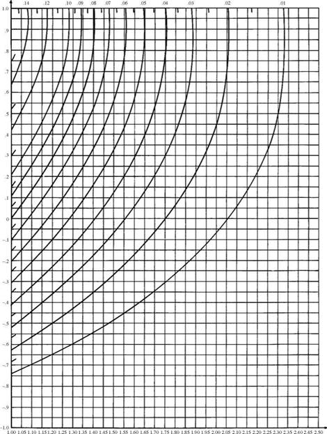
L(a, 0ip) for a > 1 and -1 < p < 1.
Values for a < 0 can be obtained using L(a, 01-p) = 0.5 – L(-a, 0lp)
Solution Based on the given information, the correlation coefficient between X1 and X2 is
Cov( X ь X2) 3.6 n„
P1,2 = ————————- = r – r – = 0.6
&X2 V9v4
Then
 P(X! < 13, X2 < 3) = PIZ! < 13 – 10, Z2 < 3-5
= P(Zi < 1, Z2 < -11 P1,2 = 0.6) = ф(а = 1, b = -11 P12 = 0.6)
By Eq. (2.118),
 Ф(1,-1|0.6) = -1 + Ф(1) + Ф(-1) + Д1, —1|0.6) Since ab = -1 < 0, according to Eq. (2.117),
,|й6)=К Чж)+К-Чж)- 2
= Д1, 0 | 0.894) + Д-1, 0 | 0.894) – 0.5
From Fig. 2.28b, Д1, 0 | 0.894) = 0.159. Since Д-1, 0 | 0.894) = 0.5 – L(1, 0 | -0.894), and according to Fig. 2.28a, by extrapolation, Д1, 0 | —0.894) = 0.004,
Д-1,0 | 0.894) = 0.5 – 0.004 = 0.496
Consequently, Д1, -11 0.6) = 0.159 + 0.496 – 0.5 = 0.155.
According to (a), the bivariate normal probability is Ф(1, -11 0.6) = Д1, -11 0.6) = 0.155. Alternatively, the bivariate normal probability can be computed by Eq. (2.121), and the result of the numerical integration for this example is 0.1569.
Multivariate normal probability. Johnson and Kotz (1976) show that if the correlation coefficient pij can be expressed as pij = XiXj for all i and j and |Xj | < 1, then each correlated standard normal random variable Zk can be represented by
Zk = Xk Z0 + J1 – Zk for k = 1> 2> ••• > K
where Z0, Z1, Z2,…, Z’Kare independent standard normal variables. The inequality Zk < zk can be expressed as
iyl zk – Xkz0
Zk < —/
Then the multivariate normal probability can be calculated as
As can be seen from Eq. (2.120), the computation of the multivariate normal probability is reduced from multiple integrals to a single integral for which the result can be obtained accurately by various numerical integration techniques. (see Appendix 4A) Under the special case of equicorrelation, that is, ptj = p, for all i and j, the multivariate normal probability can be computed as
This equation, in particular, can be applied to evaluate the bivariate normal probability.
Under the general unequal correlation case, evaluation of multivariate normal probability by Eq. (2.120) requires solving for K A’s based on K(K – 1)/2 different values of p in the correlation matrix Rx. This may not necessarily be a trivial task. Ditlevsen (1984) proposed an accurate algorithm by expanding Ф(г | Rx) in a Taylor series about an equal correlation pij = p > 0, for i = j. The equicorrelation p is determined in such a way that the first-order expansion term dФ(z | p) vanishes. The term dФ(z | p) can be expressed as
(2.122)
and Apij = pij – p. In computing the value of d Ф^ | p), numerical integration generally is required. However, one should be careful about the possible numerical overflow associated with the computation of ak (u) as the value of u gets large. It can be shown that by the L’Hospital rule, limu^TO ak(u) = 0 and
limu^-TO ak (u) = u.
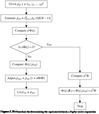
Determination of the equicorrelation p for the expansion point can be made through the iterative procedure, as outlined in Fig. 2.29. A sensible starting value for p is the average of pij:
 — 2
— 2
p = K (K – 1) ^ pij
KJ
Once such p is found, Ditlevsen (1984) suggests that the value of Ф(г | Rx) can be estimated accurately by a second-order approximation as
Ф(г |Rx) ^ Ф(г | p) + 1 d2Ф(г | p) (2.125)
in which Ф(г | p) is computed by Eq. (2.121), and the second-order error term is computed as
KKKK
 (u)aj (u)a, r (u)as(u)(—br )Sir (—bs)SjsApij Aprs
i = 1 j = 1 r = 1 s = 1
(2.126)
where Sir is the Kronecker’s delta, having a value of 1 if i = r and otherwise 0, and
As can be seen, the evaluation of Ф(z |Rx) is reduced from a multiple integral to a single integral, which can be executed efficiently and accurately by many numerical integration algorithms.
For the univariate normal distribution, an asymptotic expansion of Ф(гО is (Abramowitz and Stegun, 1972) for z
(2.128)
This expansion for Ф(z) is smaller than every summand with an odd number of terms and is larger than every summand with an even number of terms. The truncation error decreases as the number of terms increases. Note that Eq. (2.128) is particularly appropriate for evaluating the normal tail probability. The expansion has been generalized by Ruben (1964) for the multivariate normal distribution as
in which the coefficients ak are elements in a vector a obtained from
 a= Rx 1z
It should be noted that Eq. (2.130) is valid only when all coefficients ak are positive. The right-hand-side of Eq. (2.129) provides an upper bound for the multivariate normal probability.






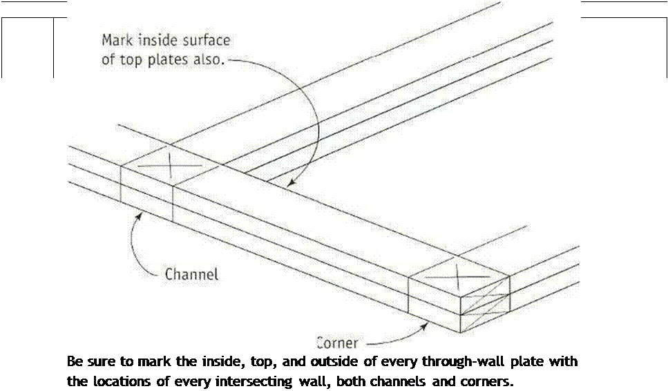


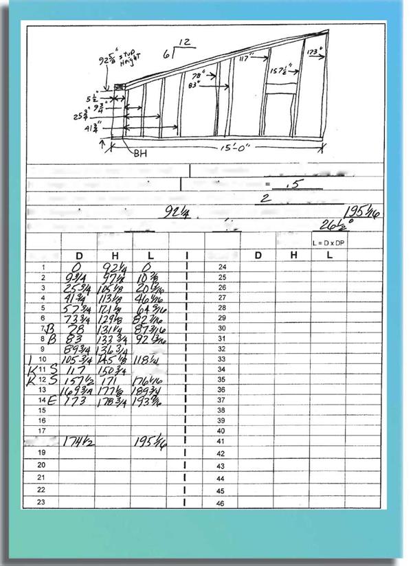
 corners and channels so you’ll have space on which to nail door and window trim. In hurricane and earthquake /ones, exterior walls must not have window or door openings less than 4 ft. from an exterior corner.





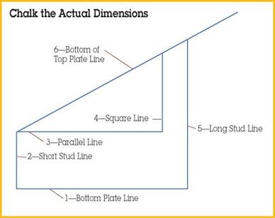 Chalk a square line (4) to the parallel line that is close to the long stud line (5), but convenient for figuring its length. The length of the square line (4) will be in a relationship to the parallel line (3), depending on the pitch of the rake wall. If, for example, the pitch is 6/12 and the parallel line is 12, the square line will be 6.
 A typical beginning height would be slightly lower than the adjoining wall, as shown in the "Rake Wall Beginning Stud Height" drawing.
 The stud height to the short point is found by using the formula (D x RP) + BH. RP is the rise percent, or the relationship between the rise and the run. The relationship gives you the height increase of the studs per increase in the distance of the plate. This relationship is illustrated in the filled-in version of the Rake Wall Stud Heights Worksheet. The formula for finding RP is also shown, in the "Rise & Diagonal Percent" illustration later in this chapter.