Multivariate lognormal distributions

Подпись: f X1,X2( x1> x2) Подпись: 1 X1 x2^ln xi ^ln x2 Подпись: , exp 1 — PH Подпись: —Q' 2(1 — pH) Подпись: (2.134)

Similar to the univariate case, bivariate lognormal random variables have a PDF

Подпись: Q' Multivariate lognormal distributions Multivariate lognormal distributions

for x1, x2 > 0, in which

where pln x and ulnx are the mean and standard deviation of log-transformed random variables, subscripts 1 and 2 indicate the random variables X1 and X2, respectively, and p12 = Corr(ln X1, lnX2) is the correlation coefficient of the two log-transformed random variables. After log-transformation is made, prop­erties of multivariate lognormal random variables follow exactly as for the multivariate normal case. The relationship between the correlation coefficients in the original and log-transformed spaces can be derived using the moment­generating function (Tung and Yen, 2005, Sec. 4.2) as

Multivariate lognormal distributions

exp (p12°ln x1 Vln x2) 1

7exp «xj — Vexp ^J — 1


Corr( X1, X 2) = P12


(2.135)


Example 2.23 Resolve Example 2.21 by assuming that both X1 and X2 are bivariate lognormal random variables.

Solution Since X1 and X2 are lognormal variables,

Подпись: = P Подпись: ln(13) - » 1 ln(3) - ix'2 Z1 < 1 , Z2 < 1 Подпись: P

P(X1 < 13, X2 < 3) = P [ln(X1) < ln(13), ln(X2) < ln(3)]

in which »2, a1, and are the means and standard deviations of ln(X1) and ln(X2), respectively; p’ is the correlation coefficient between ln(X1) and ln(X2). The values of »1, »2, a1, and 02 can be computed, according to Eqs. (2.67a) and (2.67b), as

o’x = ] ln(1 + 0.32) = 0.294 e’2 = J ln( 1 + 0.42) = 0.385

p! x = ln(10) – 2(0.294)2 = 2.259 » = ln(5) – 1(0.385)2 = 1.535

Based on Eq. (2.71), the correlation coefficient between ln(X 1) and ln(X2) is

Подпись: 0.623ln[1 + (0.6)(0.3)(0.4)]

Подпись: P = ■(0.294)(0.385)

Then

P(X1 < 13, X2 < 3 | p = 0.6) = P(Z1 < 1.04, Z2 < -1.13 | p’ = 0.623)

= Ф(а = 1.04, b = -1.13 | p’ = 0.623)

Подпись: Problems
From this point forward, the procedure for determining Ф(а = 1.04, b = -1.13 | p’ = 0.623) is exactly identical to that of Example 2.21. The result from using Eq. (2.121) is 0.1285.

2.1 Referring to Example 2.4, solve the following problems:

(a) Assume that P(.Ё!!^) = 1.0 and P(E2ІE1) = 0.8. What is the probability that the flow-carrying capacity of the sewer main is exceeded?

(b) If the flow capacity of the downstream sewer main is twice that of its two upstream branches, what is the probability that the flow capacity of the downstream sewer main is exceeded? Assume that if only branch 1 or branch 2 exceeds its corresponding capacity, the probability of flow in the sewer main exceeding its capacity is 0.15.

(c) Under the condition of (b), it is observed that surcharge occurred in the downstream sewer main. Determine the probabilities that (i) only branch 1 exceeds its capacity, (ii) only branch 2 is surcharged, and (iii) none of the sewer branches exceed their capacities.

2.2 Referring to Example 2.5, it is observed that surcharge occurred in the down­stream sewer main. Determine the probabilities that (a) only branch 1 exceeds its flow-carrying capacity, (b) only branch 2 is surcharged, and (c) none of the sewer branches exceed their capacities.

2.3 A detention basin is designed to accommodate excessive surface runoff temporar­ily during storm events. The detention basin should not overflow, if possible, to prevent potential pollution of streams or other receiving water bodies.

For simplicity, the amount of daily rainfall is categorized as heavy, moderate, and light (including none). With the present storage capacity, the detention basin is capable of accommodating runoff generated by two consecutive days of heavy rainfall or three consecutive days of moderate rainfall. The daily rainfall amounts around the detention basin site are not entirely independent. In other words, the amount of rainfall on a given day would affect the rainfall amount on the next day.

Let random variable Xt represent the amount of rainfall in any day t. The transition probability matrix indicating the conditional probability of the rainfall amount in a given day t, conditioned on the rainfall amount of the previous day, is shown in the following table.

Xt+1 =

H

M

L

H

0.3

0.5

0.2

II

$

0.3

0.4

0.3

L

0.1

0.3

0.6

(a) For a given day, the amount of rainfall is light. What is the probability that the detention basin will overflow in the next three days? (After Mays and Tung, 1992.)

(b) Compute the probability that the detention basin will overflow in the next three days. Assume that at any given day of the month the probabilities for having the various rainfall amounts are P(H) = 0.1, P(M) = 0.3, P (L) = 0.6.

2.4 Before a section of concrete pipe of a special order can be accepted for installation in a culvert project, the thickness of the pipe needs to be inspected by state high­way department personnel for specification compliance using ultrasonic reading. For this project, the required thickness of the concrete pipe wall must be at least 3 in. The inspection is done by arbitrarily selecting a point on the pipe surface and measuring the thickness at that point. The pipe is accepted if the thickness from the ultrasonic reading exceeds 3 in; otherwise, the entire section of the pipe is rejected. Suppose, from past experience, that 90 percent of all pipe sections manufactured by the factory were found to be in compliance with specifications. However, the ultrasonic thickness determination is only 80 percent reliable.

(a) What is the probability that a particular pipe section is well manufactured and will be accepted by the highway department?

(b) What is the probability that a pipe section is poorly constructed but will be accepted on the basis of ultrasonic test?

2.5 A quality-control inspector is testing the sample output from a manufacturing pro­cess for concrete pipes for a storm sewer project, wherein 95 percent of the items are satisfactory. Three pipes are chosen randomly for inspection. The successive

quality evaluations may be considered as independent. What is the probability that (a) none of the three pipes inspected are satisfactory and (b) exactly two are satisfactory?

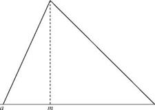
2.6 Derive the PDF for a random variable having a triangular distribution with the lower bound a, mode m, and the upper bound b, as shown in Fig. 2P.1.

2.7 Show that F 1(sq) + F2(x^) – 1 < F^xb x2) < min[F1(x1), F2(x2)]

2.8 The Farlie-Gumbel-Morgenstern bivariate uniform distribution has the following joint CDF (Hutchinson and Lai, 1990):

Fx, y(x, y) — xy [1 + в(1 – x)(1 – y)] for 0 < x, y < 1

with —1 < в < 1. Do the following exercises: (a) derive the joint PDF, (b) obtain the marginal CDF and PDF of X and Y, and (c) derive the conditional PDFs fx(x|y) and fy(y|x).

2.9 Refer to Problem 2.8. Compute (a) P(X < 0.5, Y < 0.5), (b) P(X > 0.5, Y > 0.5), and (c) P(X > 0.5 | Y = 0.5).

2.10 Apply Eq. (2.22) to show that the first four central moments in terms of moments about the origin are

Подпись: =0 _ ’ 2 — M2 Mx = M3 3MX M2 + 2MX — M4 — 4MX М3 + 6M2 М2 — 3M4 M1 М2 М3 М4

Multivariate lognormal distributions

Figure 2P.1 Triangular distribution.


b


2.11 Apply Eq. (2.23) to show that the first four moments about the origin could be expressed in terms of the first four central moments as

m1 = Mx

/ _ ,2 M2 — М2 + Mx

M3 = M3 + 3Mx М2 + m3

M4 = M4 + 4Mx М3 + 6m2 m2 +

2.12 Based on definitions of a – and ^-moments, i. e., Eqs. (2.26a) and (2.26b), (a) derive the general expressions between the two moments, and (b) write out explicitly their relations for r = 0,1, 2, and 3.

2.13 Refer to Example 2.9. Continue to derive the expressions for the third and fourth L-moments of the exponential distribution.

2.14 A company plans to build a production factory by a river. You are hired by the company as a consultant to analyze the flood risk of the factory site. It is known that the magnitude of an annual flood has a lognormal distribution with a mean of 30,000 ft3/s and standard deviation 25,000 ft3/s. It is also known from a field investigation that the stage-discharge relationship for the channel reach is Q = 1500H14, where Q is flow rate (in ft3/s) and H is water surface elevation (in feet) above a given datum. The elevation of a tentative location for the factory is 15 ft above the datum (after Mays and Tung, 1992). (a) What is the annual risk that the factory site will be flooded? (b) At this plant site, it is also known that the flood-damage function can be approximated as

n і – (Нпппч_/0 if H < 15 ft

Damage (in $1000) = |40(lnh + 8)(lnH — 2.7) if H > 15 ft

What is the annual expected flood damage? (Use the appropriate numerical ap­proximation technique for calculations.)

2.15 Referring to Problem 2.6, assume that Manning’s roughness coefficient has a triangular distribution as shown in Fig. 2P.1. (a) Derive the expression for the mean and variance of Manning’s roughness. (b) Show that (i) for a symmetric triangular distribution, a = (b — m)/V6 and (ii) when the mode is at the lower or upper bound, a = (b — a)/3 V2.

2.16 Suppose that a random variable X has a uniform distribution (Fig. 2P.2), with a and b being its lower and upper bounds, respectively. Show that (a) E (X) = xx = (b + a)/2, (b) Var(X) = (b — a)2/12, and (c) ^x = (1 — a/мх)/V3.

2.17 Referring to the uniform distribution as shown in Fig. 2P.2, (a) derive the expres­sion for the first two probability-weighted moments, and (b) derive the expressions for the L-coefficient of variation.

2.18 Refer to Example 2.8. Based on the conditional PDF obtained in part (c), de­rive the conditional expectation E(Y | x), and the conditional variance Var(Y |x).

Подпись: .Ш
Подпись: 1/(b - a)
Подпись: a Figure 2P.2 Uniform distribution.
Подпись: > x
Подпись: b

Furthermore, plot the conditional expectation and conditional standard deviation of Y on x with respect to x.

2.19 Consider two random variables X and Y having the joint PDF of the following form:

fx, y(X, y) = c (5 – 2 + x2) for 0 < x, y < 2

(a) Determine the coefficient c. (b) Derive the joint CDF. (c) Find fx (x) and fy( y).

(d) Determine the mean and variance of X and Y. (e) Compute the correlation coefficient between X and Y.

2.20 Consider the following hydrologic model in which the runoff Q is related to the rainfall R by

Q = a + bR

if a > 0 and b > 0 are model coefficients. Ignoring uncertainties of model coeffi­cients, show that Corr( Q, R) = 1.0.

2.21 Suppose that the rainfall-runoff model in Problem 2.4.11 has a model error, and it can expressed as

Q = a + bR + є

in which є is the model error term, which has a zero mean and standard deviation of ає. Furthermore, the model error є is independent of the random rainfall R. Derive the expression for Corr( Q, R).

2.22 Let X = X1 + X3 and Y = X2 + X3.FindCorr(X, Y), assuming that X1, X2, and X3 are statistically independent.

2.23 Consider two random variables Y1 and Y2 that each, individually, is a linear function of two other random variables X1 and X2 as follows:

Y1 = anX 1 + a12X 2 Y2 = a21X 1 + a>22X2

It is known that the mean and standard deviations of random variable Xk are and ffk, respectively, for k = 1, 2. (a) Derive the expression for the correlation

coefficient between Y]_ and Y2 under the condition that X1 and X2 are statistically independent. (b) Derive the expression for the correlation coefficient between Y1 and Y2 under the condition that X1 and X2 are correlated with a correlation coefficient p.

2.24 As a generalization to Problem 2.23, consider M random variables Y1, Y2,…, Ym that are linear functions of K other random variables X1, X2,…, Xk in a vector form as follows:

Ym = X for m = 1,2,…, M

in which X = (X1, X2,…, Xk)t, a column vector of K random variables Xs and aim = (am1, am2,…, amK), a row vector of coefficients for the random variable Ym. In matrix form, the preceding system of linear equations can be written as Y = AtX. Given that the mean and standard deviations of the random variable Xk are i^k and Ok, respectively, for k = 1,2,…, K, (a) derive the expression for the correlation matrix between Ys assuming that the random variable Xs are statis­tically independent, and (b) derive the expression for the correlation coefficient between Y s under the condition that the random variable Xs are correlated with a correlation matrix Rx.

2.25 A coffer dam is to be built for the construction of bridge piers in a river. In an economic analysis of the situation, it is decided to have the dam height designed to withstand floods up to 5000 ft3/s. From flood frequency analysis it is estimated that the annual maximum flood discharge has a Gumbel distribution with the mean of 2500 ft3/s and coefficient of variation of 0.25. (a) Determine the risk of flood water overtopping the coffer dam during a 3-year construction period.

(b) If the risk is considered too high and is to be reduced by half, what should be the design flood magnitude?

2.26 Recompute the probability of Problem 2.25 by using the Poisson distribution.

2.27 There are five identical pumps at a pumping station. The PDFs of the time to fail­ure of each pump are the same with an exponential distribution as Example 2.6, that is,

f (t) = 0.0008 exp(-0.0008t) for t > 0

The operation of each individual pump is assumed to be independent. The system requires at least two pumps to be in operation so as to deliver the required amount of water. Assuming that all five pumps are functioning, determine the reliability of the pump station being able to deliver the required amount of water over a 200-h period.

2.28 Referring to Example 2.14, determine the probability, by both binomial and Pois­son distributions, that there would be more than five overtopping events over a period of 100 years. Compare the results with that using the normal approxima­tion.

2.29 From a long experience of observing precipitation at a gauging station, it is found that the probability of a rainy day is 0.30. What is the probability that the next year would have at least 150 rainy days by looking up the normal probability table?

2.30 The well-known Thiem equation can be used to compute the drawdown in a con­fined and homogeneous aquifer as

in which Sik is drawdown at the ith observation location resulting from a pumpage of Qk at the kth production well, rok is the radius of influence of the kth production well, rik is the distance between the ith observation point and the kth production well, and T is the transmissivity of the aquifer. The overall effect of the aquifer drawdown at the ith observation point, when more than one production well is in operation, can be obtained, by the principle of linear superposition, as the sum of the responses caused by all production wells in the field, that is,

K K

si ‘У ‘sik ‘У ‘hikQk

k = 1 k = 1

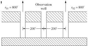
where K is the total number of production wells in operation. Consider a sys­tem consisting of two production wells and one observation well. The locations of the three wells, the pumping rates of the two production wells, and their zones of influence are shown in Fig. 2P.3. It is assumed that the transmissivity of the aquifer has a lognormal distribution with the mean гт = 4000 gallons per day per foot (gpd/ft) and standard deviation от = 2000 gpd/ft (after Mays and Tung, 1992). (a) Prove that the total drawdown in the aquifer field also is lognormally distributed. (b) Compute the exact values of the mean and variance of the total drawdown at the observation point when Q1 = 10, 000 gpd and Q2 = 15, 000 gpd.

(c) Compute the probability that the resulting drawdown at the observation point does not exceed 2 ft. (d) If the maximum allowable probability of the total draw­down exceeding 2 ft is 0.10, find out the maximum allowable total pumpage from the two production wells.

2.31 A frequently used surface pollutant washoff model is based on a first-order decay function (Sartor and Boyd, 1972):

Mt = M0e-cRt
Multivariate lognormal distributions
where M0 is the initial pollutant mass at time t = 0, R is runoff intensity (mm/h), c is the washoff coefficient (mm-1), Mt is the mass of the pollutant remaining

on the street surface (kg), and t is time elapsed (in hours) since the beginning of the storm. This model does not consider pollutant buildup and is generally appropriate for the within-storm event analysis. Suppose that M0 = 10, 000 kg and c = 1.84/cm. The runoff intensity R is a normal random variable with the mean of 10 cm/h and a coefficient of variation of 0.3. Determine the time t such that P(Mt/M0 < 0.05) = 0.90.

2.32 Consider n independent random samples X1, X2,…, Xn from an identical dis­tribution with the mean /xx and variance a2. Show that the sample mean Xn = ^2П= 1 Xi/n has the following properties:

2

E (Xn) = Px and Var( Xn) = ^

n

What would be the sampling distribution of Xn if random samples are normally distributed?

2.33 Consider that measured hydrologic quantity Y and its indicator for accuracy S are related to the unknown true quantity X as Y = SX. Assume that X ~ LN(px, ax), S ~ LN(ps = 1, as), and X is independent of S. (a) What is the distribution function for Y? Derive the expressions for the mean and coefficient of variation of Y, that is, py and Qy, in terms of those of X and S. (b) Derive the expression for rp = yp /xp with P(Y < yp) = P(X < Xp) = p and plot rp versus p. (c) Define measurement error as є = Y — X. Determine the minimum reliability of the measurement so that the corresponding relative absolute error |є/X| does not exceed the require precision of 5 percent.

2.34 Consider that measured discharge Q’ is subject to measurement error є and that both are related to the true but unknown discharge Q as (Cong and Xu, 1987)

Q = Q + є

It is common to assume that (i) E(є | q) = 0, (ii) Var^ | q) = [a(q)q]2, and (iii) ran­dom error є is normally distributed, that is, є | q ~ N(рє | q = 0, ає q).

(a) Show that E(Q’ | q) = q, E [(Q’/Q) — 11 q] = 0, and Var[( Q’/Q — 1)2 | q] = a2(q).

(b) Under a(q) = a, showthat E (Q’) = E (Q),VarW = a2 E (Q2),andVar( Q’) = (1 + a2)Var( Q) + a2 E 2( Q). (c) Suppose that it is required that 75 percent of measure­ments have relative errors in the range of ±5 percent (precision level). Determine the corresponding value of a(q) assuming that the measurement error is normally distributed.

2.35 Show that the valid range of the correlation coefficient obtained in Example 2.20 is correct also for the general case of exponential random variables with parameters в1 and @2 of the form of Eq. (2.79).

2.36 Referring to Example 2.20, derive the range of the correlation coefficient for a bivariate exponential distribution using Farlie’s formula (Eq. 2.107).

2.37 The Pareto distribution is used frequently in economic analysis to describe the randomness of benefit, cost, and income. Consider two correlated Pareto random
variables, each of which has the following marginal PDFs:

adk

fk (xk) = — xk >dk > 0 a > 0, for k = 1,2

xk

Derive the joint PDF and joint CDF by Morgenstern’s formula. Furthermore, derive the expression for E(X1X2) and the correlation coefficient between X1 and X2.

2.38 Repeat Problem 2.37 using Farlie’s formula.

2.39 Analyzing the stream flow data from several flood events, it is found that the flood peak discharge Q and the corresponding volume V have the following relation­ship:

ln(V) = a + b x ln( Q) + є

in which a and b are constants, and є is the model error term. Suppose that the model error term є has a normal distribution with mean 0 and standard deviation ає. Then show that the conditional PDF of V | Q, h(v |q), is a lognormal distribution. Furthermore, suppose that the peak discharge is a lognormal random variable. Show that the joint PDF of V and Q is bivariate lognormal.

2.40 Analyzing the stream flow data from 105 flood events at different locations in Wyoming, Wahl and Rankl (1993) found that the flood peak discharge Q (in ft3/s) and the corresponding volume V (in acre-feet, AF) have the following relation­ship:

ln(V) = ln(0.0655) + 1.011 x ln( Q) + є

in which є is the model error term with the assumed ає = 0.3. A flood frequency analysis of the North Platte River near Walden, Colorado, indicated that the annual maximum flood has a lognormal distribution with mean xq = 1380 ft3/s and ffQ = 440 ft3/s. (a) Derive the joint PDF of V and Q for the annual maximum flood. (b) Determine the correlation coefficient between V and Q. (c) Compute P(Q > 2000 ft3/s, V > 180 AF).

2.41 Let X2 = <0) + a1 Z1 + 02 Z2 and X2 = b0 + b1 Z2 + b2 Z^ in which Z1 and Z2 are

bivariate standard normal random variables with a correlation coefficient p, that is, Corr(Z1, Z2) = p. Derive the expression for Corr(X1, X2) in terms ofpolynomial coefficients and p.

2.42 Let X1 and X2 be bivariate lognormal random variables. Show that

Подпись: < Corr(X1, X2)

Multivariate lognormal distributions Multivariate lognormal distributions Подпись: 1

exp ( tfln X1 tfln X2) 1

Multivariate lognormal distributions Multivariate lognormal distributions Подпись: 1

exp aln x1 aln x2 – 1

What does this inequality indicate?

2.43 Derive Eq. (2.71) from Eq. (2.135):

Подпись: ln(1 + pi2^i^2) y/ln(l + n2^/in(i +Corr(lnXi, lnX2) = pi2

where pi2 = Corr(Xi, X2) and ^ = coefficient of variation of Xk, k = i, 2.

2.44 Develop a computer program using Ditlevsen’s expansion for estimating the mul­tivariate normal probability.

2.45 Подпись: References
Develop computer programs for multivariate normal probability bounds by Rack – witz’s procedure and Ditlevsen’s procedure, respectively.

Abramowitz, M., andStegun, I. A., eds. (i972). Handbook of Mathematical Functions with Formulas,

Determination of bounds on multivariate normal probability

Instead of computing the exact value of Ф(z |Rx), several methods have been proposed to determine the bounds on the exact value of Ф(z |Rx). This section describes three such bounds.

Bounds of Rackwitz. The scheme of Rackwitz (1978) is based on the decompo­sition of a positive correlation coefficient pij = XiXj, for i, j = 1, 2,…, K. The multivariate normal probability Ф(z |Rx) is obtained according to Eq. (2.120). Instead of solving for the exact values for all K(K – 1)/2Xs, Rackwitz selects the smallest three values of z = (z1, z2,…, zK)* in Ф^ |Rx) and solves for the corresponding Xs that satisfy pij = XiXj, for i, j = [1], [2], [3] with subscript [i]
representing the rank of zs in ascending order, that is, Z[p < Z[2] < Z[3] <• ■ ■ < zyK-i] < Z[K]. For example, assume that all ptj s are positive. Based on the three smallest zs, one can solve for X[i] for i = 1, 2, 3 in terms of рщ[j] as

Determination of bounds on multivariate normal probability

P[1][2] P[1][3]
P[2][3]


1/2


P[1][2] P[2][3]
P[1][3]


1/2


P[1][3] P[2][3]
P[1][2]


1/2


X[1]


X[2]


X[3]


(2.131)

Determination of bounds on multivariate normal probability Подпись: i = [4], [5], ...,[K ] i = [4], [5], ...,[K ] Подпись: (2.132a) (2.132b)

For the remaining Xs, their values can be computed as

The upper bound and lower bound of Ф(z |Rx) can be obtained by Eq. (2.120) along with Xs computed by Eqs. (2.132a) and (2.132b), respectively.

Подпись: ФL(z |Rx) = Ф^1) -^2 max I Ф(-Zk) - max |>(-Zk, -Zj | pkj)] / k 2 j < k Подпись: (2.133a)

Подпись: K Фи(z |Rx) = Ф^1) -^2 max ^ 0, k = 2 K Determination of bounds on multivariate normal probability
Подпись: j = 1

Bounds of Ditlevsen. Ditlevsen (1979) proposed an approach for the bounds of the multivariate normal probability as follows:

(2.133b)

in which Фи (z | Rx) and Ф^ | Rx) are the upper and lower bounds of the multi­variate normal probability, respectively, and Ф(zk, Zj | pkj) is the bivariate nor­mal probability. Ditlevsen (1979) further simplified these bounds to involve the evaluation of only the univariate normal probability at the expense of having a more complicated algebraic expression where a narrow bound can be obtained under |p | < 0.6. For a larger correlation coefficient, Ditlevsen (1982) proposed a procedure using conditioning to obtain a narrow bound. The derivations of various probability bounds for system reliability are presented in Sec. 7.2.5

1.00

0.80

0.64

0.51

0.41

0.80

1.00

0.80

0.64

0.51

0.64

0.80

1.00

0.80

0.64

0.51

0.64

0.80

1.00

0.80

0.41

0.51

0.64

0.80

1.00

Example 2.22 Z1, Z2, Z3, Z4, and Z5 are correlated standard normal variables with the following correlation matrix:

Rx —

Determine the multivariate probability P (Zi < -1, Z2 < —2, Z3 < 0, Z4 < 2, Z5 < 1) by Ditlevsen’s approach using the Taylor series expansion. Also compute the bounds for the preceding multivariate normal probability using Rackwitz’s and Ditlevsen’s approaches.

Solution Using Ditlevsen’s Taylor series expansion approach, the initial equicorrela – tion value can be used according to Eq. (2.124) as p = 0.655. The corresponding mul­tivariate normal probability, based on Eq. (2.121), is Ф(г | p = 0.655) = 0.01707. From Eq. (2.122), the first-order error, d Ф(г | p = 0.655), is 0.003958. Results of iterations according to the procedure outlined in Fig. 2.29 are shown below:

i

p

Ф(2|p)

dФ(г|p)

1

0.6550

0.01707

0.3958 x 10—2

2

0.8069

0.02100

—0.1660 x 10—3

3

0.8005

0.02086

—0.3200 x 10—4

4

0.7993

0.02083

—0.5426 x 10—5

At p = 0.7993, the corresponding second-order error term in the Taylor series ex­pansion, according to Eq. (2.126), is

d2Ф(г| p) = 0.01411

Based on Eq. (2.125), the multivariate normal probability can be estimated as Ф(z| Rx) = Ф(г| p = 0.7993) + 0.5d2Ф(г| p = 0.7993)

= 0.02083 + 0.5(0.01411)

0.02789

Using the Rackwitz approach for computing the bounds of the multivariate normal probability, the values ofzs are arranged in ascending order as (гщ, Z[2], Z[3], Z[4], Z[5]) = (—2, —1, 0,1, 2) = (Z2, Z1, Z3, Z5, Z4) with the corresponding correlation matrix as

1.00

0.80

0.80

0.51

0.41

0.80

1.00

0.64

0.41

0.51

0.80

0.64

1.00

0.64

0.80

0.51

0.41

0.80

1.00

0.80

0.64

0.51

0.80

0.80

1.00

R[kj]

The values of ks corresponding to the three smallest zs, that is, —2, —1, and 0, are computed according to Eq. (2.131), and the results are

k[1] = 1.00 k[2] = 0.80 k[3] = 0.80

Using Eq. (2.132a), the values of the remaining ks for computing the upper bound are obtained as

Determination of bounds on multivariate normal probability

Determination of bounds on multivariate normal probability Determination of bounds on multivariate normal probability

k[4]u = max


1.00


k[5],U = max


and, by the same token, for the lower bound are

k[4], l = 0.51 X[5], l = 0.6375

Applying Eq. (2.120), along with Хц = (1.0, 0.8, 0.8, 0.8, 1.0), one obtains the upper bound for the multivariate normal probability Фц(z |Rx) = 0.01699. Similarly, using Xl = (1.0, 0.8, 0.8, 0.51, 0.6375), the lower bound is obtained as ФL(z |Rx) = 0.01697.

To use Eqs. (2.133a) and (2.133b) for computing the upper and lower bounds for the multivariate normal probability, the marginal probabilities and each pair of bivariate normal probabilities are computed first, according to Eq. (2.3). The results are

Ф(г1) = 0.1587 Ф( z2) = 0.02275 Ф(г3) = 0.5000 Ф( z4) = 0.9772 Ф(г5) = 0.8413

Ф(-z1, —z2) = 0.8395 Ф(-z1, —z3) = 0.4816

Ф(—z1, —z4) = 0.0226 Ф(—z1, —z5) = 0.1523

Ф(—z2, — z3) = 0.5000 Ф(—z2, —z4) = 0.0228 Ф(—z2, —z5) = 0.1585

Ф(—z3, —z4) = 0.0227 Ф(—z3, —z5) = 0.1403 Ф(—z4, —z5) = 0.0209

The lower and upper bounds of the multivariate probability can be obtained as 0.02070 and 0.02086, respectively.

MAKING A STORY POLE

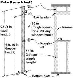
Подпись: 61/4 in. (top cripple length) Подпись: Make a story pole from a 2x stud. This pole will help you accurately lay out trimmers, headers, rough sills, and top and bottom cripples.The best way to obtain accurate lengths for cripples and trimmers is to make a story pole. As the name suggests, this straight length of wood (I use a 2×4) tells a story. In this case, it’s the description of a wall layout, with the locations of sills and headers for win­dows and doors providing the measurements for cutting cripples and trimmers. With a story pole, you do all the measuring once, double-check everything, then use the pole as a reference for the entire layout. Instead of repeatedly measuring cripples and trim­mers with a tape measure, you simply transfer the layout marks from the story pole.

To make a story pole, select a straight stud and nail a short scrap of 2×4 on one end to act as the bottom plate. Then, mea­suring upward from the base of the bottom plate, clearly mark the underside of the header at 6 ft. 10 in. (assuming that is the header height). Measure upward another 1У2 in. for a single flat header, 3У2 in. for a 4×4 header, and 5V2 in. for a 4×6 header, mak­ing clear marks across the story pole. The distances remaining above the header layout lines are the lengths of the top cripples. Remember that headers for pocket and bifold doors may be high­er, so their cripples will be shorter. Label the layout lines on your story pole to avoid confusion.

To locate windowsills, measure the window height down from the bottom of the header. Measure down another 1У2 in. for a single 2x rough sill. The amount remaining is the length of the bottom cripples. The trimmer lengths are measured from the bot­tom plate to the bottom of the header.

the way in which headers will be constructed. A good way to carry around this information is with a story pole, as explained in the sidebar above. Recording wall-building information on a story pole reduces the chance of error and speeds the entire framing process.

Determine dimensions for stud length and header height

Stud length, header height, and other “stan­dard” dimensions vary somewhat from region to region. Find out what is standard in your area. Out west, where I’m accustomed to
framing, we use a stud that is 921/4 in. long. Headers for doors and windows are usually held 6 ft. 10 in. off the subfloor. Check the height in your region, though—in some places, the stan­dard is 6 ft. 10V2 in. Headers for pocket doors and closet bifold doors may need to be higher to allow room for an overhead track. Door and window sizes are noted on the plans with des­ignations such as 3/0 x 6/8 (36 in. by 80 in.) or 5/0 x 4/0 (60 in. by 48 in.). Carpenters will say, “There’s a three-oh by six-eight door,” or “We’ve got a five-oh by four-oh window going in this wall.” The first measurement is the width, the

Post and Beam Frame

The “beam” component of “post and beam” timber framing usually refers to a heavy top plate, sometimes called a girt, or it could refer to a girder. Girts will often be supported later by infilling the individual panels of the building’s perimeter. In this book, I use the word “panel” to refer to the spaces between posts around the perimeter. Girts can also gain strength by the use of intermediate posts, between the major posts. If not called upon to provide a joining surface for two consecutive girts, these intermediate posts can be less substantial, thus less expensive. An example of this is our garage at Earthwood. See Figures 2.12 (photo) and 2.13 (post and girt plan.) We have full-sized eight-by-eights at each corner of the 24-foot by 28-foot (7.3-meter by 8.5-meter) structure. In addition, we have eight-by-eights halfway along the walls. But, providing further strength to the girts, we have what I think of as secondary posts, still substantial four by-eights, laid up so that the eight-inch (20.3 centimeter) dimension corresponds with the 8-inch thickness of the wall. The sides of the building, therefore, have four panels

on the long side, each about seven feet in length including the posts, and also four panels on the south (gable) side, each about six feet long. The 24-foot­wide north side features a 16-foot garage door, with little four-foot panels on each side. An 18-foot-long (5.48- meter) eight-by-eight carries the girt system over the garage door. This large beam can also be thought of as a giant lintel over the garage door.

I was told at a building supply that the rough opening for our double garage door was 8 feet high and 16 feet wide, and it was framed accordingly. In reality, the height dimension turned out to be seven, not eight, feet (2.13 meters). The door fit with a foot to spare. We later hung a horizontal two-

by-eight from the eight-by eight with 10-inch pieces of two-by-eight material, filling the spaces with cordwood masonry. Because of this mistake, our garage is actually a foot higher than it needed to be, causing me to do a bit of extra cordwood work.

In the case of the girts at our garage, they were well-supported during construction, with temporary diagonals screwed to the external frame to prevent racking of the building due to wind loads. Later, individual diagonals would be removed and panels would be filled in with cordwood masonry, which also serves to prevent racking. We do not have any true girders at our garage, as we have at the Earthwood house. It is the clear-span girders in a post and beam frame that need to be engineered for both shear and bending. Appendix В gives an example of this.


Safety practices on the job site

• Take a course in basic first aid.

• Watch out for your fellow worker. Be aware of who is nearby so you don’t hit someone with a piece of lumber or with your hammer.

• Try to have a good, positive attitude.

• Keep your work area clean. It’s easy to trip over scrap wood, lumber, tools, and trash.

• Pull or bend over nails that are sticking out of boards so nobody gets injured.

• Spread sand on ice in winter to provide traction.

• Don’t turn the radio up so loud that you can’t hear other workers. Concentration and communication on the job site are critical to avoiding accidents.

• Concentrate on the task at hand.

• Work at a steady, careful pace.

• Back injuries are very common on the job. To pre­serve your back, remember to lift with your legs, not with your back.

• Take care of your body by eating good food and exercising. And don’t forget to rest. Getting enough sleep is important to keeping your concentration and to avoiding fatigue.

• Take a break when you feel tired. Don’t overwork yourself. Exhaustion leads to carelessness.

• Don’t drink or take drugs while working. Operating power tools under the influence is as dangerous as driving under the influence.

• Watch where you walk, especially when working on scaffolds or on the frame of the house. Many in­juries on the job are the result of falls.

• Follow your instinct. If something you are about to do feels unsafe, it probably is. Pay attention to the voice inside your head when it says, “Be careful.”

degree of skill. Still, installing a prehung door requires attention to detail, which is why I’ll discuss the process more in Chapter 8. I’ll also talk about how to install a lockset.

Exterior and interior trim

Trimming out a house is like adding the frosting to a birthday cake. Whether you are installing exterior or interior casing, sills, aprons, or baseboard, there’s a wide variety of styles and profiles from which to choose—from simple 1×4 trim to ornate crown moldings.

Clear stock is pricey, but it’s ideal for trim because it can be stained, left unfinished, or painted with little prepa­ration. Finger-jointed stock (short pieces glued together) is less expensive than clear stock but needs to be painted to cover the joints (that’s why it’s called paint-grade trim). Knots aren’t an insur­mountable problem as long as they are sound and won’t fall out, and trim can be preprimed so that the knots won’t bleed pitch through the paint.

Exterior casing around doors and win­dows not only serves a functional purpose but also adds beauty and char­acter. Look at houses as you drive around your neighborhood and note all of the different kinds of trim. Check out the vertical boards nailed to the corners. See the casings that go around doors and windows. Fascia boards are nailed to rafter tails to give them a finished look. Frieze boards are nailed between rafters to seal them off. All of this exte­rior trim can be as simple as a plain 1×4 or as elaborate as the filigree that you

The maritime civilizations of the Aegean Sea: urban and agricultural hydraulics

The first great European civilizations are found in and on the shores of the Aegean Sea – and thus in direct maritime contact with Egypt and Syrian ports. The earliest such civilizations are the Cyclades thalassocracy in the IIIrd millennium BC, the first mar­itime power of the Mediterranean; then Minoan Crete beginning at the end of the IIIrd millennium BC.[137] Civilization flourishes all around the Aegean Sea during the IInd millennium BC – especially in Crete, but also on the island of Cyprus, and in Asia Minor, with Troy to the north, and to the south Rhodes, Samos, and Kos. The first Hellenes came to continental Greece in several waves, and it is very likely around 1900 BC that Greek-speaking people appear – the Acheans. The warrior civilization that we call the Mycenaen developed from this time. Maritime trade is particularly active during this entire period – among all the European civilized lands, of course, but also with Syria, including the port of Ugarit to the north on the trade routes to Mari and to Hattusha, the capital of the Hittite Empire; and the port of Byblos to the south, threshold to Egypt.

The maritime civilizations of the Aegean Sea: urban and agricultural hydraulics

New arrivals from the north appear between 1200 and 1100 BC: the Dorians. This begins the disappearance of the Mycenaen civilization, whose survivors desert the cities.

Some flee to the islands and coast of Asia Minor (Ionia). This is possibly the origin of the “Sea People” that we met in Chapter 2, responsible for the burning and sometimes the disappearance of the main cites of Levant. The destruction of Troy is likely one of the episodes of this drama. In the Ionian islands, the memory of the bellicose Acheans is preserved in the Homeric poems the Iliad and the Odyssey.

Lumber dimensions

When ordering lumber or making plans for anything built with wood, it’s important to remember that the lumber designation (2×4, 4×4, 1×8, etc.) is not the actual lumber size. For instance, a 2×4 is not really 2 in. by 4 in., and a 1×8 is not really 1 in. by 8 in. (this is called the nominal dimension).

In general, rough lumber stock (2xs, 4xs, 6xs, etc.) is V2 in. under the nominal size (all lumber lengths are actual, however). For instance, a 2×4 is actually 11/2 in. thick and 31/г in. wide. For 1x stock, however,
the actual dimensions are a bit different. A 1×8, for example, is 3A in. thick (1A in. under the nominal size) and 71/2 in. wide (V2 in. under the nominal size).

Manufactured lumber can be designated by the ac­tual dimensions. A 3/4-in.-thick 4×8 sheet of OSB is just that: 3A in. thick and 4 ft. wide by 8 ft. long. A 6×12 laminated beam, on the other hand, will usual­ly measure 5Уг in. by 111/2 in. When buying these items, check their dimensions to see if they meet your actual needs.

Lumber dimensions

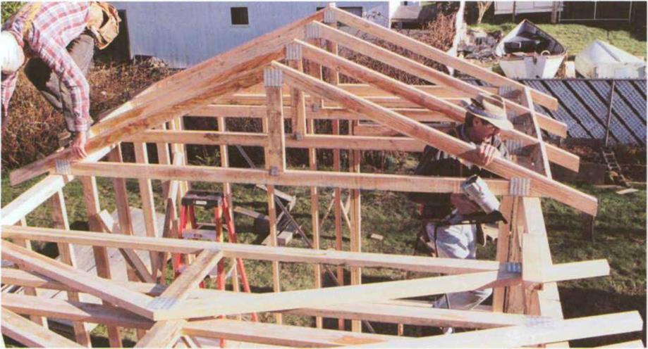
Roof trusses, which are delivered to the site fully assembled, simplify roof construction. Notice the frieze blocks (on right) between these king-post trusses, which help tie the whole roof together. (Photo by Roe A. Osborn.)


the frame of a house has to be struc­turally strong, but it doesn’t have to be free of knots. Clear, knot-free lumber is desirable for finish work because it looks the best. Unfortunately, clear lum­ber has become increasingly expensive because of the depletion of our old – growth forests, so choosing finish lumber often involves sorting through stacks of boards.

In the western part of the country, construction-grade Douglas fir and hem­lock are the preferred framing woods. In other parts of the country, selected species of pine or spruce are strong enough to support a house frame.

Clear-grade finish lumber in almost any species is available at a premium price. Popular species such as redwood, pine, and oak are available in more economi­cal grades. I prefer the No. 2 stock over

clear grades. The cheaper grade may be harder to work, but knots add character and interest to a board.

I am a carpenter, so I love the feel of real wood. It’s sad that the old-growth trees are gone, because the new, fast-growing trees have little structural strength.

Many are cut into chips to make manu­factured lumber.

Manufactured lumber

Manufactured lumber products are being used for sheathing, joists, and beams. Manufactured sheathing prod­ucts include plywood, OSB, and medium-density fiberboard (MDF).

These sheet goods are available in various thicknesses, from 1A in. to 3A in. and thicker.

Plywood is made by gluing and pressing thin layers of veneer together. Construction-grade exterior plywood

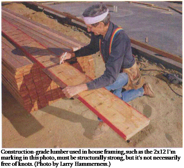
Подпись: Construction-grade lumber used in house framing, such as the 2x12 I'm marking in this photo, must be structurally strong, but it's not necessarily free of knots. (Photo by Larry Hammerness.) (CDX) is made from thin layers of fir or other common softwoods glued together with a waterproof glue so it can be used on the building exterior.
OSB and MDF are made by compressing and gluing strands or particles of wood fiber to create panels. Structurally rated OSB is used for exterior sheathing, while MDF makes a good substrate for things like countertops and closet shelves. Be careful when working with MDF. The substance bonding the wood fibers may contain formaldehyde, and the dust from cutting it is fine, like flour. It’s a good idea to wear a respirator (which is much more effective than a dust mask) when cutting this material, unless you are working outside in a stiff wind.

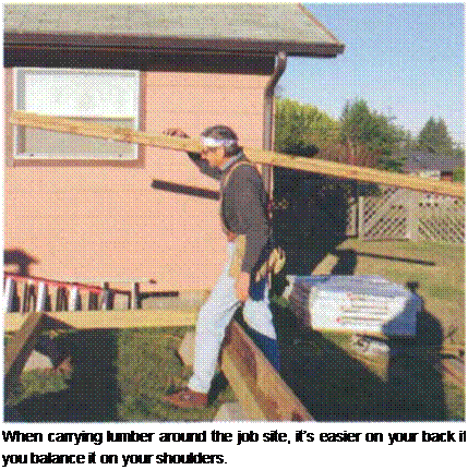
Подпись: When carrying lumber around the job site, it’s easier on your back if you balance it on your shoulders.

Подпись: CARRYING LUMBER
Подпись: Much of the lumber used in frame carpentry is heavy. To avoid hurting your back, learn to lift with your legs and arms, and learn how to carry lumber around properly. If you carry lumber with your hands at your waist, you may strain your lower back. It’s better to carry boards on your shoulder, where the backbone, rather than the back muscles, supports the weight. When you need to carry a long, heavy 2x rafter or joist, grab it at its balance point near the center and lift it in one easy motion, flipping it so that it lands gently on your shoulder. Then it’s simply a matter of balancing the board as you walk, rather than wrestling with it. Don’t get into a strength contest. If something is too heavy to carry by yourself comfortably, ask another person for help, or make more trips with smaller loads. A strained back is no joke.

Becoming more common in house con­struction are wooden I-beam joists (see Sources on p. 198) made with a ply-

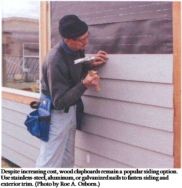
Подпись: Despite increasing cost, wood clapboards remain a popular siding option. Use stainless-steel, aluminum, or galvanized nails to fasten siding and exterior trim. (Photo by Roe A. Osborn.) wood strip (called a web) glued into flanges at top and bottom (see the photo on p. 67). These joists are light­weight and can span long distances, making it possible to create very large rooms. Also, they are always straight and don’t shrink as much as 2x joists, so floors tend to remain flat, level, and rela­tively squeak free.

Engineered beams are typically made from laminated strips of lumber. These are available in several widths and depths and can span distances upwards of 60 ft. without support. A 31/2-in.-wide beam can be used as a header in a 2×4 wall. Engineered beams are stable, which means they won’t twist and split the way regular 2x or 4x lumber does.

Siding

A builder friend of mine here in wet, coastal Oregon was showing me a new house that was lap-sided with new – growth cedar clapboards. He told me that 25 years ago the old-growth cedar trees had 20 growth rings to the inch, while today the new-growth trees have around three rings to the inch. Almost every board on the house he showed me was cupped.

Quality wood siding that will stay flat on a building is expensive and hard to find. Because of this, wood clapboards —-though still popular—-face stiff com­petition from alternative siding products. Today, builders are siding houses with aluminum and vinyl, composite materials like plywood, boards made of pressed wood fibers (OSB), or even material with a cement-fiber content.

While some of these materials—like syn­thetic or natural stucco—are applied by specialty subcontractors, cutting and fit­ting siding is typically a job for a carpenter. Siding must protect the build­ing from sun and rain and make the house look good, so I’ll devote more time to installing it later on in Chapter 8.

Windows, doors, and trim

When I was growing up, we forced strips of cloth around all the window sash with a kitchen knife when the weather got cold to plug the cracks around the loose-fitting windows. What a pleasure it is now to have tight-fitting, insulated windows and doors to keep out the cold.

When carpenters talk about windows and doors, you’ll hear them say "a three-oh by four-oh unit" (3/0 x 4/0). They are talking about a window that is 3 ft. wide by 4 ft. high. The width is given first and the height second. A 2/8 x 6/8 ("two-eight by six-eight") door is 32 in. wide by 80 in. high.

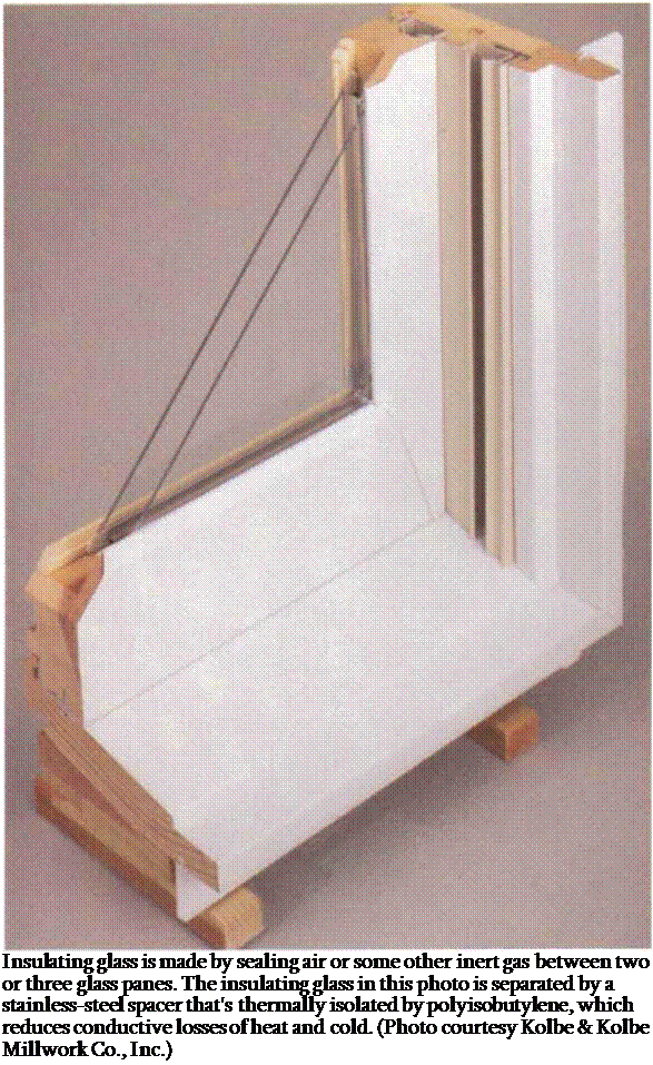
Подпись: Insulating glass is made by sealing air or some other inert gas between two or three glass panes. The insulating glass in this photo is separated by a stainless-steel spacer that's thermally isolated by polyisobutylene, which reduces conductive losses of heat and cold. (Photo courtesy Kolbe & Kolbe Millwork Co., Inc.) Windows When I first started building, we had basically one choice for win­dows: wood framed. Although wood-framed windows are still around, other options are available now in a wide variety of styles.
Vinyl – and aluminum-framed windows are sold everywhere. Vinyl frames cut down on condensation in cold or humid
climates. Both frames are basically main­tenance free, requiring just an occasional washing. Aluminum-framed windows are less expensive than vinyl and come in different colors (most vinyl­framed windows are white).

Windows with double glazing (called insulated glass) have two or three panes of glass with a sealed airspace between them (see the photo at left). The air­space keeps the window free from condensation and cuts down on heat loss in the winter, helping to keep the cold—and the noise—outside.

Among the dozens of window styles, the most commonly used are fixed, slid­ing, double hung, and single hung. A fixed window is just a frame with glass. Sliding windows have fixed glass on one side and a frame that slides back and forth on the other side. A double-hung unit has a bottom and top sash, both of which can be moved up or down.

A single-hung unit also has a bottom and top sash, but only the bottom sash can be opened.

Doors Doors have also changed a lot since I first started building. Now there are molded wood-product interior doors with a hollow core, genuine frame-and – panel interior and exterior doors, doors sheathed with metal or fiberglass over a wood frame and an energy-efficient foam core, and elaborate hardwood doors with etched glass, often with a solid core. Doors come in a wide range of prices and quality and are available either individually or as prehung units.

Prehung doors come already mounted in their jambs, have a threshold and weatherstripping (if it’s an exterior door), and often even have holes bored for the lockset and dead bolt. These units radi­cally simplify door installation because you don’t have to make the jambs or mount the door on its hinges, a time – consuming process that takes a high

FRAMING

Framing a roof is the most difficult aspect of framing, and the ability to construct a roof is a real test of your framing skills. This chapter has three separate sections. The first addresses basic rafter framing, including roof framing terms, roof styles, five methods of finding rafter lengths, the eleven steps for framing a roof with rafters, and ceiling joist information.

The second section of the chapter covers finding rafter lengths using the “Diagonal Percent" method. You can follow an example to learn how to cut difficult rafters. If you master this system, you will be able to “cut and stack" a roof, which means you can cut all the rafters and stack them ready for installation before the first one is installed. If you are familiar with the basics of rafter cutting, you might want to skip to this section. Some of the basic steps are duplicated for the example. The final section of the chapter discusses the eight steps of roof truss framing.

Roof trusses are typically pre-manufactured off site and delivered to the job site. They are engineered for strength and use standard dimension lumber. Gang nail plates are used to connect the cords and struts that make up the trusses.

The angles and pitches of a roof are as varied as the colors in a child’s crayon box. Just as some colors

have certain characteristics in common, so do rafters and trusses. This chapter is organized around these common characteristics. Key steps for framing a roof with rafters and trusses are provided.

The most difficult part of framing a roof is finding the rafter length. It is based on the relationship between the rise (vertical) distance and the run (horizontal) distance. In this chapter, you’ll find methods for finding the rafter length, though you ultimately will only need to memorize the approach you’re most comfortable with. You will also find that at different times you might want to use different methods.

Prefabricated trusses, factory-made from the architect’s specifications, require, of course, no calculations on your part. Uniform in size, they are somewhat easier to work with than ridgeboards and rafters. Still, they are heavy to work with, especially working at heights.

This chapter starts with important rafter terms, followed by steps for calculating and cutting rafters and installing sheathing. The second half of the chapter provides more detailed information and examples on finding rafter length. The chapter ends with a discussion of joists and trusses.

Roof Framing Terms

Hip rafter

Important Rafter Terms

Span—the distance between two supporting members, typically measured from the outside of two bearing walls.

Run—horizontal distance.

Rise—vertical distance.

Diagonal—the distance between the far point on the run and the high point on the rise. (Similar to hypotenuse in mathematical terms.)

Hip or valley run—the horizontal distance below the hip or valley of a roof, from the outside corner of the wall to the center framing point.

Overhang hip run—the horizontal distance below the overhang hip of the roof, from the outside corner of the wall to the outside corner of the fascia.

Hip or valley diagonal—the distance between the far point on the hip or valley run and the high point on the hip or valley rise.

Overhang diagonal—the distance between the far point on the overhang run and the high point on the overhang rise.

Diagonal percent—the diagonal divided by the run.

Hip-val diagonal percent—the hip or valley diagonal divided by the hip or valley run.

Rise percent—the rise divided by the run.

Pitch—the slope of the roof, or the relationship of the run to the rise. Typically defined as a certain height of rise for 12 units of run for a common rafter, and 17 (16.97) units of run on a 90° hip or valley rafter.

Framing point—the point where the center lines of connecting rafters, ridges, hips, or valleys would meet.

Cheek cut—an angle cut that is made to bear against another rafter, hip, or valley.

Common rafter—a rafter running from a wall straight to a ridge board.

Jack rafter—a rafter running to a hip rafter or a valley rafter.

Hip rafter—a rafter at an outside corner of a roof that runs in between and joins jack rafters that bear on corner walls.

Valley rafter—a rafter at an inside corner of a roof that runs between and joins with jack rafters from each side.

Ridge end rafter—a rafter that runs from the end of a ridge.

Pitch angle—the vertical angle on the end of a rafter that represents the pitch of the roof.

Connection angle—the horizontal angle at the end of a rafter needed to connect to other rafters, hips, valleys, or ridge boards.

Techniques BLOCKING IN BATHROOMS AND CLOSETS

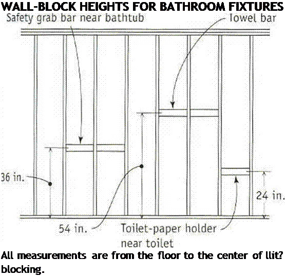
Подпись: WALL-BLOCK HEIGHTS FOR BATHROOM FIXTURES All measurements are from the floor to the center of llit? blocking. Подпись: Many fixtures in a bathroom require solid blocking behind the drywall to ensure safe, secure mounting.

NAILED BETWEEN STUDS, blocking provides solid backing for items such as towel racks, closet shelves, and safety grab bars. Blocking ensures that the mounting hardware for those devices can be anchored with screws driven into solid wood, so that you don’t have to worry about racks, bars, and shelves pulling loose.

It’s smart to include blocking when marking up wall plates. Cut blocking boards from 2x scraps. As shown in the illustration below, blocking is installed

so that the face of the 2x is flush with the edges of the studs. To help locate blocking, use these stan­dard heights for common bath, kitchen, and storage fixtures:

* Towel bars: Block near the tub and vanity and center 54 in. above the floor.

^ Toilet-paper holder: Block near the toilet and center 24 in. above the floor.

a Toothbrush and soap holder: Block above the sink and center 40 in. above the floor.

^ Safety grab bars: Block near the toilet and near (or in) the bathtub/shower and center 36 in. above the floor.

a Closet shelf and pole: Block 66 in. above the floor; more blocking may be needed if you install wire shelves.

^ Linen-closet shelves: First block above the floor at 20 in., then block every 14 in. thereafter for above-floor measurements of 34 in., 48 in.,

62 in., and 76 in. Don’t forget to block for a shelf or two in the utility room to hold detergent and other laundry items.

ж Kitchen cabinets: Block below 36 in. for base cabinets, above 54 in. and below 84 in. for wall cabinets.

a Shutters: Block at the top and bottom of windows at least 12 in. wide.

tub trap. Measure 15 in. from the wall to the center of the tub trap and make a mark. Then measure 6 in. to each side of the mark (for a 12-in. hole) and strike lines onto the plates. MarkaiTT’bn the outside of these lines on both plates to show the studs’ positions.

Once a tub/shower unit has been installed, plumber will nail it in place to a harking Stud. Measure 32 in. from the corner and mark both plates with keel. The stud location is away from this mark. Toward the inside,
mark the location of a flat stud that will be nailed to the first stud. T he flat stud provides backing for the tub.

Plans often show an in-wall medicine cabi­net (MC) centered over the bathroom sink. The standard rough opening for an in-wall medicine cabinet is 1414 in. wide. To accom­modate one, measure 7/ in. in each direction from the center (directly over the sink’s drain pipe) and mark across both plates with keel, making an “X” on the outside of each line to

STREETS

Streets are an integral part of neighborhoods, and must be designed to provide adequate access to individual lots with minimal interference in the daily lives of residents. Wide pavements and rights-of-way occupy land which could be used to increase housing density or as open space. Following are guidelines for local streets:

• Limit right-of-way widths to the minimum necessary for street construction and maintenance.

• Use easements rather than rights-of-way for sidewalks and utilities.

• Design streets for their anticipated use.

• Coordinate street widths with the number of travel lanes and amount of parking necessary.

• Reduce pavement thickness, where possible, to match structural design with actual performance needs of subdivision streets.

• Reduce the traditional radius requirements for "bulb" cul-de-sacs, or substitute hammerheads, T-turnarounds, and islands.

R. O.W.

S/W.

s/w^

w ції ї(мгіч= in in»*»ч а і*2-*гіи ; hi • «ги< *’и aiui wi*tu її

і s«<i * їм * in»uu«i**a; k<

Typical right-of-way

Подпись: Rights-of-Way and EasementsRights-of-way are publicly-owned land on which streets, sidewalks, curbs, and gutters are built, and which often accommodate utilities such as water, sewer, and electrical service. The government body that owns the right – of-way grants the right of use and passage to the public, or to designated parties such as utilities, under conditions specified by the govern­ment. Right-of-way land is not on the property tax rolls and generates no tax income.
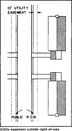
Easements are rights of passage and/or use on property that remains in private ownership. In residential situations, the owners of easement land are homeowners, and the holder of the easements is the utility company or municipality. The municipality prescribes types and conditions of use of easements, as it does for rights-of-way. The satne access to utilities is available as when utilities are installed in rights – of-way. Easement land is taxable.

STREETSПодпись: Advantages of Easement UsageUse of easements as an alternative to rights-of-way provides benefits to each of the parties involved in residential development.

The municipality gains:

• Additional land on the tax rolls

• Reduction in land for which it has responsibility of maintenance

The builder gains:

• More land to sell

• Increased design flexibility

The homeowner gains:

• More usable land

• Lower home costs

Jurisdictions routinely specify a minimum right-of-way width of 50 feet or greater, which comprises sufficient width for a roadway 30 to 36 feet wide, with broad margins for sidewalks and utilities. Such specifications reflect a past era of lower land values. In today’s environment, they should be subjected to rigorous review to reduce housing costs.

Подпись: Right-of-Way Width The basic facility that must be accommodated by a right-of-way is the roadway with its associated shoulders, curbs, and gutters. As discussed below, traditional designs often resulted in streets much wider than were necessary. This was done for two reasons:

• Detailed planning to relate road width to reasonable anticipated usage was usually not carried out.

• Substantial road capacity was routinely built to allow for unevaluated possibilities of "future growth."

The first step in reducing right-of-way width is substituting detailed traffic analysis and planning for general guidelines, and applying this planning to the width of residential roadways and connecting streets.

STREETS

Street without sidewalks


Sidewalks located outside right-of-way

Other uses of rights-of-way, including sidewalks, placement of utilities, snow storage space, and planting strips, should be evaluated. One alternative is to accommodate uses other than roads with easements. If easements cannot be used for such applications, right-of-way requirements for them often can be reduced, as discussed in ensuing sections.

Several configurations are illustrated with different ROW limits. Each varies according to the pavement width, the sidewalk placement, utility strips, and other related items.

Подпись: Street DesignState highway standards often serve as a basis for local street standards. However, traffic characteristics, _ construction and maintenance require­ments, and performance needs of residential streets differ from those of highways. Reductions in cost and in land use can be achieved by

designing residential streets so as not to exceed these characteristics, requirements, and needs. This will often involve departure from es­tablished criteria and practices which are based on broad application of general rules rather than individual analysis.

Подпись: Pavement Width Local construction standards often specify a minimum pavement width of 30 to 36 feet, an excessive amount of space for most residential streets. Depending on such factors as speed limit, parking requirements, and lane width, street pavement widths can be reduced to as narrow as 18 feet.
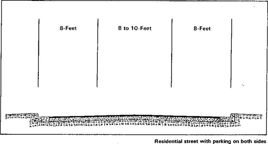
Such narrower streets will effectively and safely accommodate the relatively low speed limits appropriate for subdivisions.

The number of lanes and their width are the primary factors upon which pavement width should be based. Eight feet is usually adequate for parking lanes, with moving lanes requiring 8 to 10 feet depending on individual conditions. Guidelines

STREETS

published jointly by the National Association of Home Builders, the American Society of Civil Engineers, and the Urban Land Institute state that a street width of 24 feet is adequate for two parking lanes and one moving lane. On low volume, low speed streets typical in a residential neighborhood, it is not necessary to provide two unobstructed moving lanes. If two cars are parked directly across from each other, there is usually room for one moving vehicle to pull over and let the other pass. This is a minor inconvenience on a residential street and is outweighed by the savings in land, construction, and maintenance costs.

STREETS
Pavement widths can be narrowed further by eliminating one or both parking lanes. Rural streets and collector streets that do not provide direct access to homes are not used for parking and do not require a pavement width greater than that which will allow two cars to pass. Pavement widths of 18 to 20 feet are adequate for such roads.

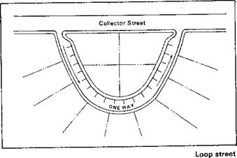
Подпись: LoopsLoop streets can reduce costs, especially if designed for one-way’ traffic. A 16- to 18-foot pavement on

a one-way loop will accommodate both moving traffic and a lane of parked cars, as illustrated.

The one-way loop provides two points of ingress and egress for fire equip­ment and other emergency vehicles.

Construction of a safe, durable roadway is a function of traffic volume, of the weight of vehicles expected to use the roadway, and of underlying soil conditions.

State highway departments generally prescribe minimum standards for state roads regarding the thickness of pavements and construction materials and methods. These standards are for roads that will ordinarily carry heavier vehicles and more traffic than expected on subdivision streets. However, many municipalities and local governments adopt standards for subdivision streets that reflect those for state roads. Significant cost savings can be realized by substituting analysis of the actual functional requirements of subdivision streets.

A minimum thickness of 8 to 12 inches for the base layer of crushed stone aggregate, or other material underlying the paved road surface, is not an uncommon requirement for residential streets. Consideration can be given to reducing the thickness of the base layer to match actual functional requirements, as was done in the Lacey, Washington, affordable housing project, as shown.

Подпись: Intermediate Asphalt Applications and Surface CoursesSTREETS
Local aggregates for the base layer are often available at lower cost than typical crushed stone bases. Such materials should be used when possible. ‘

Intermediate asphalt applications, usually a carry-over from highway construction practices, can be elimi­nated from most subdivision street designs. Because the major contribu­tion to pavement stability is provided by the underlying base layer and subgrade, a single 1 1/2-inch to 2-inch surface course, depending on the size of the aggregate in the asphalt, is usually adequate.

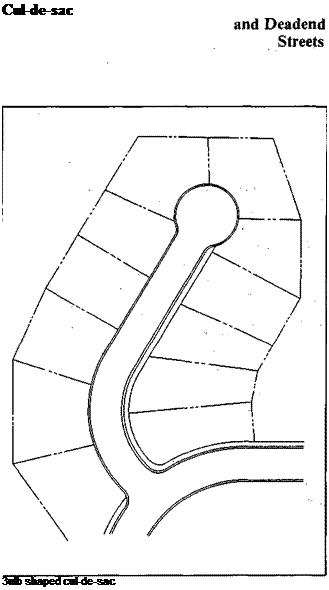
Подпись: Cul-de-sac 3ulb shaped cul-de-sac In addition to savings from adoption of functional construction criteria, other savings can be achieved through modification of certain features of layout and design.

Alternative designs for the traditional large "bulb-shaped" cul-de-sac can be cost effective. Many communities require that cul-de-sacs have a radius of 50 to 60 feet. However, 35 to 40 foot cul-de-sacs are adequate in most residential settings.

Large cul-de-sacs are often adopted at the urging of fire officials to assure an adequate turning radius for fire­fighting equipment. In some instances, requirements of this type have been in effect for substantial periods of time and reflect the time when fire trucks did not have reverse gears. However, 50 feet significantly exceeds the turning radius of modern compact fire trucks. Communities with very large trucks should consider more compact equipment at replacement time, both for direct savings and for additional savings through the adoption of more economical street designs.

STREETS
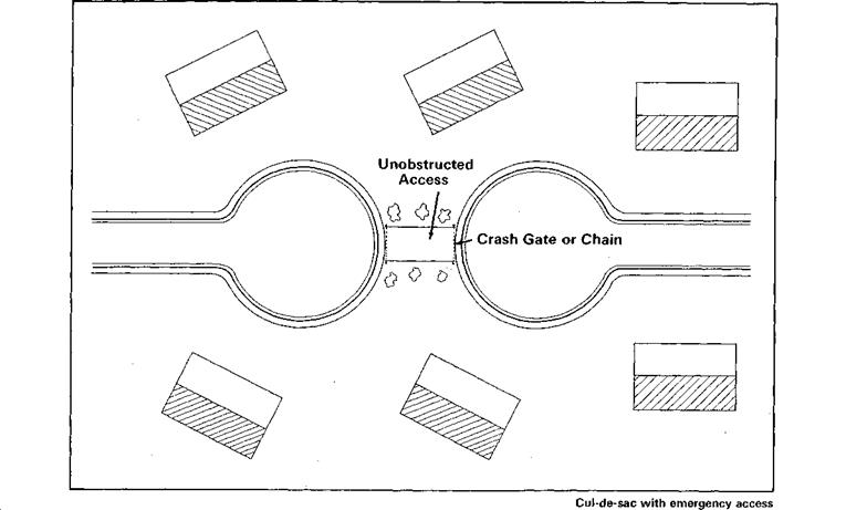
Cul-de-sacs and deadend streets can be laid out "back to back" with a short intervening space between them over which the municipality has an easement for use as emergency access. The concept of emergency access can also be applied to deadend streets that have been narrowed as a cost saving measure. Property owners should not be permitted to install any type of fencing, planting, or landscaping that would form a serious barrier to emergency vehicles.

Подпись: Hammerheads, T-Turnarounds, Islands STREETS
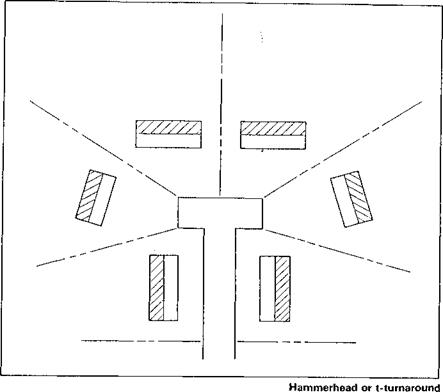
Other cost-saving alternatives to the traditional bulb-shaped cul-de-sac include the hammerhead or T-turnaround, and islands. Both configurations require significantly less pavement than is required for bulb cul-de-sacs and a narrower right-of – way.