Category Hydrosystems Engineering Reliability Assessment and Risk Analysis

Bounds for system reliability

Despite the system under consideration being a series or parallel system, the evaluation of system reliability or failure probability involves probabilities of union or intersection of multiple events. Without losing generality, the deriva­tion of the bounds for P (A1U A2 U—U AM) and P (A1 n A2 П—П AM) are given below.

For example, consider P(A1 U A2 U-U AM). When Am = Fm, the probability is for the failure probability of a series system, whereas when Am = Fm, the probability is for the reliability of a parallel system. The bounds of system failure probability, that is, can be defined as follows:

Pf ,sys – Pf, sys – Pf, sys (7.11a)

with p f sys and p f, sys being the lower and upper bounds of system failure prob­ability, respectively. The corresponding bounds for system reliability can be obtained as

1 – Pf, sys = PS, SyS – Ps, sys – Ps, sys = 1 – Pf, sys (7.11b)

Similarly, after the bounds on system reliability are obtained, the bounds on system failure reliability can be computed easily.

First-order bounds. These bounds also are called unimodal bounds (Ang and Tang, 1984, p. 450). They can be derived as follows. Referring to Eq. (2.7), the probability of the joint occurrence of several events can be computed as

P ( П A^ = P (A1) x P (A2 | A1) x—x P ( Am | Am-1, Am-2, ■ ■■, A2, A1)

m=1 )

(7.12)

Under the condition that all events Aj and Am are positively correlated, the following inequality relationship holds:

P (Am | Aj ) > P (Am)

Hence

P (Aj, Am) = P (Am | Aj)P ( Aj ) > P ( Am)P (Aj )

This can be extended to a multiple-event case as

Bounds for system reliability

M

П Am

m=1


P


(7.13)


m1


Bounds for system reliability

As can be seen, the lower bound of the probability of an intersection is when all events are as if they are independent. Furthermore, it is also true that

П Am c Aj for any j = 1, 2, ■■■, M

m=1

Therefore,

Подпись: M , П Am m1 c min{ A1, A2, ■■■, Am }

Подпись: P Подпись: M Am Подпись: - min{P(A1), P(A2), ■■■, P(AM)} Подпись: (7.14)

Consequently,

Подпись: M П P (Am ) < P m=1 Подпись: M П Am m1 Подпись: < min {P (Am)} m=1,2,..., M Подпись: (7.15)

Based on Eqs. (7.13) and (7.14), the bounds on probability of joint occurrence of several positively correlated events are

Example 7.3 Consider three standardized normal random variables Z1, Z2, and Z3 with the following correlation matrix:

1.000

0.841

0.014

Rz =

0.841

1.000

0.536

0.014

0.536

1.000

Compute the first-order bounds for P{(Z1 < —2.71) U (Z2 < —2.88) U (Z3 < —3.44)}.

Solution The three events corresponding to the preceding trivariate normal probability are

A1 = {Z1 < -2.71} A2 = {Z2 < -2.88} A3 = {Z3 < -3.44}

Since,

P(A1 U A2 U A3) = 1 — P(Aj П A П A3)

the first-order bounds for P( A1U A2 U A3) can be obtained from those of P(A1П A П A3).

To derive the first-order bounds for P(A1 П A П A3), individual probabilities are required, which can be obtained from Table 2.2 or Eq. (2.63) as

P(A[) = P(Z1 > -2.71) = 0.99664

P(A2) = P(Z2 > -2.88) = 0.99801

P(A3) = P(Z3 > -3.44) = 0.99971

Furthermore, because all Am’s are positively correlated, all Am’s are also positively correlated. According to Eq. (7.15), the first-order bounds for P(A1 П A^ П A3) is

(0.99664)(0.99801)(0.99971) < P[ n Am) < min{0.99664, 0.99801, 0.99971}

m=1

Подпись: 0.99437 < P Подпись: 3 П Am m=1 Подпись: < 0.99664

which can be reduced to

Подпись: 1 - 0.99664 < P Bounds for system reliability Подпись: < 1 - 0.99437

Therefore, the corresponding first-order bounds for P(A1 U A2 U A3) is

Подпись: 0.00336 P Подпись: 3 U Am Подпись: 0.00563

which can be reduced to

Referring to Eq. (7.2), the first-order bounds for reliability of a series system with positively correlated nonfailure events can be computed as

M

П P (Fm) < ps, SyS < min{P (Fm)} (7.16a)

m=1

or in terms of failure probability as

M

IT [1 – P (Fm)] < Ps, sys < min{1 – P (Fm)} (7.16b)

m

m=1

Similarly, referring to Eq. (7.7), by letting Am = Fm, the first-order bounds on the failure probability of a parallel system with positively correlated failure events can be immediately obtained as

M

TT P(Fm) < Pf, sys < min{P(Fm)} (7.17a)

m

m=1

Bounds for system reliability Подпись: (7.17b)

and the corresponding bounds for the system reliability, according to Eq. (7.11b), is

Example 7.4 Consider that the M identical components in a system are positively correlated and the component reliability is ps. Determine the reliability bounds for the system.

Solution If the system is a series system, the bounds on system reliability, according to Eq. (7.16a), are

PM < Ps, sys < Ps

When the system is in parallel, the bounds on the system reliability, according to Eq. (7.17b), are

Ps < Ps, sys < 1 – (1 – Ps)M

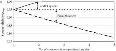
The bounds for system reliabilities for different M, with the component reliability of 0.95, for series and parallel systems are shown in Fig. 7.6. As can be observed, the bounds for the system widen as the number of components increases.

In the case that all events Am’s are negatively correlated, the following rela­tionships hold:

P (Am | Aj) < P (Aj) for all j, m

P(Aj, Am) < P(Aj )P(Am)

Hence the first-order bounds for the probability of joint occurrence of several negatively correlated events is

Подпись: M . n Am m=1 Подпись:

Bounds for system reliability

M

< П P (Am)

m=1

The bounds for reliability of a series system, with Am = F’m, containing nega­tively correlated events are

M

0 < Ps, sys < [1 – P (Fm)]

m=1

Подпись: 1

Bounds for system reliability

whereas for a parallel system, with Am = Fm,

It should be pointed out that the first-order bounds for system reliability may be too wide to be meaningful. Tighter bounds sometimes are required and can be obtained at the expense of more computations.

Second-order bounds (Bimodal bounds). The second-order bounds are obtained by retaining the terms involving the joint probability of two events. By Eq. (2.4), the probability of the union of several events is

p(u Am) = E P (Am)-EE P (Ai, Aj) + Y, P (Ai, Aj, Ak)-•••

‘ ‘ m=1 i< j i< j < k

+ (-1) MP (A1, A2,…, Am ) (7.18)

Notice the alternating signs in Eq. (7.18) as the order of the terms increases. It is evident that the inclusion of only the first-order terms, that is, P(Am), produces an upper bound for P (A1 U A2 U ■ ■ ■ U AM). Consideration of the only the first two order terms yields a lower bound, the first three order terms again an upper bound, and so on (Melchers, 1999).

Bounds for system reliability Подпись: M U m=1 Bounds for system reliability Подпись: (7.19)

Simple bounds for the probability of a union are

It should be pointed out that these bounds produce adequate results only when the values of P(Am) and P(Am, Aj) are small. Equation (7.18) alternatively can be written as

P M Am) = [P (A1)] + [P (A2) – P (A1, A2)] + [ P (A3) – P (A1, A3)

m=1

— P (A2, A3) + P (A1, A2, A3)] + [P (A4) — P (A1, A4) — P (A2, A4)

— P (A3, A4) + P (A1, A2, A4) + P (A1, A3, A4) + P (A2, A3, A4)

— P (A1, A2, A3, A4)] + [P (A5) ••• (7.20)

To derive the lower bound, consider each of the terms in brackets in Eq. (7.20). For example, consider the bracket containing the terms associated with event A4. Note that apart from P(A4), the remaining terms in the bracket are

-P [(A1, A4) U (A2, A4) U (A3, A4)]

Подпись: P Bounds for system reliability Bounds for system reliability

Furthermore, event A4 contains (A1, A4)U(A2, A4)U(A3, A4), which implies that P (A4) > P [(A1, A4) U (A2, A4) U (A3, A4)]. Consequently, each of the bracketed terms in Eq. (7.20) has a nonnegative probability value. Also notice that

and thus the following inequality holds:

Подпись:Подпись: P(A4) - P3

> P(A4) – Y P (Aj, At)

j=1

This equation can be generalized as

Подпись: mU1(Aj , Am) j=1m-1

Подпись: P (Am) - P> P(Am) – Y P (Aj, Am) (7.21)

j=1

It should be pointed out that the terms on the right-hand-side of Eq. (7.21) could be negative, especially when m is large. Owing to the fact that each of the

Подпись: P Подпись: M U Am n=1 Bounds for system reliability Bounds for system reliability Подпись: 0 Подпись: (7.22)

bracketed terms should be nonnegative, abetter lower bound to Eq. (7.20) can be obtained if the right-hand-side of Eq. (7.21) makes a nonnegative contribution to the lower bound (Ditlevsen, 1979), namely,

Earlier, Kounias (1968) proposed an alternative second-order lower bound by selecting only those combinations in Eq. (7.20) which give the maximum values of the lower bound:

pQ^ Am^j > P(A1) + max J ^[P(Am) – P(Aj, Am)](7.23)

j <m J

It should be pointed out that both lower bounds for the probability of a union depend on the order in which the events are labeled. Algorithms have been de­veloped for identifying the optimal ordering of events to obtain the best bounds (Dawson and Sankoff, 1967; Hunter, 1977). A useful rule of thumb is to order the events in the order of decreasing importance (Melchers, 1999). In other words, events are ordered such that P(A[1]) > P ( A[2]) > ••• > P(A[M]), with [m] representing the rank of the event according to its probability of occurrence. For a given ordering, Ramachandran (1984) showed that the lower bound pro­vided by Eq. (7.22) is better than Eq. (7.23), whereas both bounds are equal if all possible orderings are considered.

To derive the upper bound, attention is focused back to Eq. (7.20) and on each of the terms in brackets. For example, consider the bracket containing the terms associated with event A4. As discussed earlier, apart from P ( A4), the remaining terms in the bracket are

—P [(A1, A4) U (A2, A4) U (A3, A4)]

Using the fact that P(A U B) > max[P(A), P(B)], the following inequality holds:

Подпись: PU (Aj, A4) > max[P(Aj, A4)]

Lj <4 j j <4

Bounds for system reliability Подпись: < P(A4) — max[P(Aj, A4)] (7.24) j <4

Hence the probability in the fourth bracket involving event A4 satisfies

Bounds for system reliability Подпись: (7.25)

This inequality relation is true for all the bracketed terms of Eq. (7.22), and the upper bound can be obtained as

Bounds for system reliability
Example 7.5 Refer to Example 7.3. Compute the second-order bounds for the multi­variate normal probability.

Solution To compute the second-order bounds, the probabilities of individual events as well as the joint probabilities between two different event pairs must be computed. From Table 2.2 or Eq. (2.63), the probabilities of individual events are

P(A1) = P(Z1 < -2.71) = 0.003364

P(A2) = P(Z2 < -2.88) = 0.001988

P(A3) = P(Z3 < -3.44) = 0.0002909

The joint probabilities, according to the procedures described in Sec. 2.7.2, are P(A1, A2) = P(Z1 < -2.71, Z2 < -2.88 | p = 0.841) = 0.0009247

P(A1, A3) = P(Z1 < -2.71, Z3 < -3.44 | p = 0.014) = 0.000001142

Bounds for system reliability Подпись: m-1 P(Am) -£) P(AJ , Am) J =1 Подпись: ,0

P(A2, A3) = P(Z2 < -2.88, Z3 < -3.44 | p = 0.536) = 0.00004231 The lower bound of P(A1 U A2 U A3), according to Eq. (7.23), is

= P(A1) + max{[P(A2) – P(A1, A2)], ^ + max{[P(A3) – P(A1, A2) – P(A2, Ae)],0} = 0.003364 + max[[0.001988 – 0.0009247], 0} +max{[2.909 x 10⁻⁴ – 1.142 x 10⁻⁶) -4.231 x 10⁻⁵], 0} = 0.003364 + 0.00106633 + 0.00024736 = 0.004675

The upper bound of P(Ai U A2 U A3), according to Eq. (7.25), can be computed as

3 3

V P(Am) – У max[P(Aj, Am)]

m=1 m=2

3

= У P(Am) – {max[P(A1, A2)] + max[P(A1, A3), P(A2, A3)]}

m=i

= (0.003364 + 0.001988 + 0.002909) У max(0.0009247)

+ max[(1.142 x 10⁻⁶, 4.231 x 10⁻⁵)]} = 0.005641 – (0.000924 + 0.0000425)

= 0.004677

In summary, the second-order bounds for the trivariate normal probability P (A1 U A2 U A3) are

0.004675 < P(A1 U A2 U A3) < 0.004677

Comparing with the first-order bounds obtained in Example 7.3, the second-order bounds are definitely tighter.

Basic probability rules for system reliability

The solution approaches to system reliability problems can be classified broadly into failure-modes approach and survival-modes approach (Bennett and Ang, 1983). The failure-modes approach is based on identification of all possible fail­ure modes for the system, whereas the survival-modes approach is based on the all possible modes of operation under which the system will be operational. The two approaches are complementary. Depending on the operational char­acteristics and configuration of the system, a proper choice of one of the two approaches often can lead to significant reduction in efforts needed for the re­liability computation.

Подпись: pf ,sys Подпись: P (F1 U F2 U---U FM) = P Подпись: M U Fm n=1 Подпись: (7.1)

Consider that a system has M components or modes of operation. Let event Fm indicate that the mth component or mode of operation is in the failure state. If the system is a series system, the failure probability of the system is the probability that at least one of the M components or modes of operation fails, namely,

in which pf, sys is the failure probability of the system. On the other hand, the system reliability ps, sys is the probability that all its components or modes of operation perform satisfactorily, that is,

ps, sys = P(F1 n F2 n-.-n FM) = p( n F^ (7.2)

m=1 J

in which Fm is the complementary event of Fm indicating that the mth compo­nent or mode of operation does not fail.

In general, failure events associated with system components or modes of op­eration are not mutually exclusive. Therefore, referring to Eq. (2.4), the failure

probability for a series system can be computed as

n M M_1 M

Подпись: Pf ,sys = PmUi Fm) = £ P(Fm) _^ X) P(Fi, F,)
‘ m=1 i = l j =i + 1

+ EEE P (Fi, Fj, FA ) -… + (-1) MP (Fi, F2,…, Fm ) (7.3)

i< j < Л

According to Eq. (2.7), the reliability for a series system is

Ps, sys = P (F1) X P (F2 | F1) X P (FjJ | F1, F-2) X ••• x P (FM | F1, F-2,…, FM_1)

(7.4)

In the case that failure events Fm’s are mutually exclusive or the probability of joint occurrence of multiple failures is negligible, the failure probability of a series system can be easily obtained as

M

Pf, SyS = £ P(Fm) (7.5a)

m=1

with the corresponding system reliability

M

ps, sys = 1 _ pf, sys = 1 ^ ] P (Fm) (7.5b)

m=1

Under the condition that all failure events are statistically independent, the reliability of a series system can be computed easily as

MM

Ps, SyS = П P(Fm) HI [1 _ P(Fm)] (7.6a)

m=1 m=1

with the corresponding system failure probability

M

Pf, SyS = 1 _П [1 _ P(Fm)] (7.6b)

m=1

The component probability P(Fm) can be determined by methods described in Chaps. 4, 5, and 6 of this book.

Example 7.1 Consider a series system consisting of M independent components, each with an identical component reliability of ps. The system reliability, according to Eq. (7.6a), is

n – PM

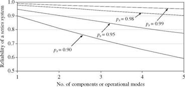
Ps, sys = P s

Figure 7.4 shows the relationship among the reliability of a series system, component reliability, and the number of components. As can be seen, the reliability of a series system decreases as the number of components increases.

Basic probability rules for system reliability

Basic probability rules for system reliability

Figure 7.4 Relationship among reliability of a series system, component reliability, and the number of components.


In the case of a parallel system, the system would fail if all its components or modes of operation failed. Hence the failure probability for a parallel system is

Pf, sys = P(F1 n F2 П—П Fm) = P П Fm (7.7)

m=1

The reliability of a parallel system, on the other hand, is the probability that at least one of its component or modes of operation is functioning, that is,

Ps, sys = P (F1 U F2U-.-U FM) = P U Fm (7.8)

m=1

Hence, under the condition of independence for all failure events, the failure probability of a parallel system simply is

M

Подпись: (7.9a)Подпись: (7.9b)pf, sys = П P (Fm)

m=1

with the corresponding system reliability being

Подпись: MM

Ps, sys = 1 – П P (Fm) = 1 – П [! – P (Fm)]

Подпись: m=1m=1

Example 7.2 Consider a parallel system consisting of M independent components, each with an identical component reliability of ps. The system reliability, according to Eq. (7.9b), is

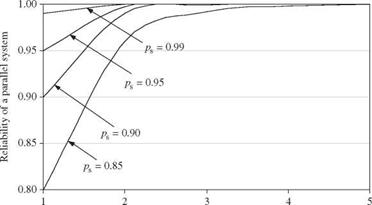
Ps, sys = 1 – (1 – Ps )M

Figure 7.5 shows the relationship among reliability of a parallel system, component reliability, and the number of components. The figure indicates that the reliability of a parallel system increases as the number of components increases.

Basic probability rules for system reliability

No. of components or operational modes

Figure 7.5 Relationship among reliability of a parallel system, component reliability, and the number of components.

For mutually exclusive failure events, reliability of a parallel system can be computed as

M M

Pssys = P (Fm) = M – P(Fm) (7.10a)

m=1 m=l

with the corresponding system failure probability

M

Pf, sys = 1 + P (Fm) – M (7.10b)

m=l

Unfortunately, for a real-life system involving multiple components or modes of operation, the corresponding failure events are neither independent nor mu­tually exclusive. Consequently, the computation of exact values of system reli­ability and failure probability would not be a straightforward task. In practical engineering applications, bounds on system reliability are computed based on simpler expressions with less computational effort. As will be seen in the next subsection, to achieve tighter bounds on system reliability or failure probability, a more elaborate computation will be required. Of course, the required preci­sion for the computed system reliability is largely dependent on the importance of the satisfactory performance of the system under consideration.

Classification of systems

From the reliability computation viewpoint, classification of the system depends primarily on how system performance is affected by its components or modes of operation. A multiple-component system called a series system (see Fig. 7.1) requires that all its components perform satisfactorily to allow satisfactory performance of the entire system. Similarly, for a single-component system involving several modes of operation, it is also viewed as a series system if satisfactory performance of the system requires satisfactory performance of all its different modes of operation.

A second basic type of system is called a parallel system (see Fig. 7.2). A parallel system is characterized by the property that the system would serve its intended purpose satisfactorily as long as at least one of its components or modes of operation performs satisfactorily.

For most real-life problems, system configurations are complex, in which the components are arranged as a mixture of series and parallel subsystems or in the form of a loop. In dealing with the reliability analysis of a complex system, the general approach is to reduce the system configuration, based on the ar­rangement of its components or modes of operation, to a simpler situation for which the reliability analysis can be performed easily. However, this goal may not always be achievable, in which case a special procedure would have to be devised.

General View of System Reliability Computation

Подпись: Figure 7.2 Schematic diagram of a parallel system.
General View of System Reliability Computation

As mentioned previously, the reliability of a system depends on the component reliabilities and interactions and configurations of components. Consequently, computation of system reliability requires knowing what constitutes the system being in a failed or satisfactory state. Such knowledge is essential for system classification and dictates the methodology to be used for system reliability determination.

General View of System Reliability Computation

Figure 7.3 Procedure for infrastructural engineering system reliability.

Reliability of Systems

7.1 Introduction

Most systems involve many subsystems and components whose performances affect the performance of the system as a whole. The reliability of the entire system is affected not only by the reliability of individual subsystems and components but also by the interactions and configurations of the subsystems and components. Many engineering systems involve multiple failure paths or modes; that is, there are several potential paths and modes of failure in which the occurrence, either individually or in combination, would constitute system failure. As mentioned in Sec. 1.3, engineering system failure can be structural failure such that the system can no longer function, or it can be performance failure, for which the objective is not achieved but the functioning of the system is not damaged. In terms of their functioning configuration and layout pattern, engineering systems can be classified into series systems or parallel systems, as shown schematically in Figs. 7.1 and 7.2, respectively.

A formal quantitative reliability analysis for an engineering system involves a number of procedures, as illustrated in Fig. 7.3. First, the system domain is defined, the type of the system is identified, and the conditions involved in the problem are defined. Second, the kind offailure is identified and defined. Third, factors that contribute to the working and failure of the system are identified. Fourth, uncertainty analysis for each of the contributing component factors or subsystems is performed. Chapters 4 and 5 of Tung and Yen (2005) and Chap. 6 of this book describe some of the methods that can be used for this step. Fifth, based on the characteristics of the system and the nature of the failure, a logic tree is selected to relate the failure modes and paths involving different com­ponents or subsystems. Fault trees, event trees, and decision trees are the logic trees often used. Sixth, identify and select an appropriate method or meth­ods that can combine the components or subsystems following the logic of the tree to facilitate computation of system reliability. Some of the computational

Copyright © 2006 by The McGraw-Hill Companies, Inc. Click here for terms of use.

Подпись: Figure 7.1 Schematic diagram of a series system.

methods are described in Chaps. 4, 5, and 6. Seventh, perform the computation following the methods selected in the sixth step to determine the system failure probability and reliability. Eighth, if the cost of the damage associated with the system failure is desired and the failure damage cost function is known or can be determined, it can be combined with the system failure probability function determined in step 7 to yield the expected damage cost.

The different contributing factors or parameters may have different measure­ment units. In quantitative combination for reliability analysis, these statistical parameters or factors are normalized through their respective mean or stan­dard deviation to become nondimensional, such as coefficients of variation, to facilitate uncertainty combination.

Real-life hydrosystems engineering infrastructural systems often are so large and complex that teams of experts of different disciplines are required to con­duct the reliability analysis and computation. Logic trees are tools that permit division of team work and subsequent integration for the system result. In­formation on the logic trees and types of systems related to steps 5 and 6 are discussed in this chapter.

Resampling Techniques

Note that the Monte Carlo simulation described in preceding sections is con­ducted under the condition that the probability distribution and the associated population parameters are known for the random variables involved in the system. The observed data are not used directly in the simulation. In many statistical estimation problems, the statistics of interest often are expressed as functions of random observations, that is,

© = ©( X1, X 2,…, Xn) (6.110)

The statistics © could be estimators of unknown population parameters of in­terest. For example, consider that random observations Xs are the annual max­imum floods. The statistics © could be the distribution of the floods; statisti­cal properties such as mean, standard deviation, and skewness coefficient; the magnitude of the 100-year event; a probability of exceeding the capacity of a hydraulic structure; and so on.

Note that the statistic © is a function of the random variables. It is also a random variable, having a PDF, mean, and standard deviation like any other

random variable. After a set of n observations {X1 = x1, X2 = x2,___________________________________________ , Xn = xn}

is available, the numerical value of the statistic © can be computed. However, along with the estimation of © values, a host of relevant issues can be raised with regard to the accuracy associated with the estimated ©, its bias, its confi­dence interval, and so on. These issues can be evaluated using the Monte Carlo simulation in which many sequences of random variates of size n are generated from each of which the value of the statistic of interest is computed ©. Then the statistical properties of © can be summarized.

Unlike the Monte Carlo simulation approach, resampling techniques are de­veloped that reproduce random data exclusively on the basis of observed data. Tung and Yen (2005, Sec. 6.7) described two resampling techniques, namely, the jackknife method and the bootstrap method. A brief description of the latter is given below because the bootstrap method is more versatile and general than the jackknife method.

The bootstrap technique was first proposed by Efron (1979a, 1979b) to deal with the variance estimation of sample statistics based on observations. The technique intends to be a more general and versatile procedure for sampling distribution problems without having to rely heavily on the normality condition on which classical statistical inferences are based. In fact, it is not uncommon to observe nonnormal data in hydrosystems engineering problems. Although the bootstrap technique is computationally intensive—a price to pay to break away from dependence on the normality theory—such concerns will be dimin­ished gradually as the calculating power of the computers increases (Diaconis and Efron, 1983). An excellent overall review and summary of bootstrap tech­niques, variations, and other resampling procedures are given by Efron (1982) and Efron and Tibshirani (1993). In hydrosystems engineering, bootstrap pro­cedures have been applied to assess the uncertainty associated with the dis­tributional parameters in flood frequency analysis (Tung and Mays, 1981), op­timal risk-based hydraulic design of bridges (Tung and Mays, 1982), and unit hydrograph derivation (Zhao et al., 1997).

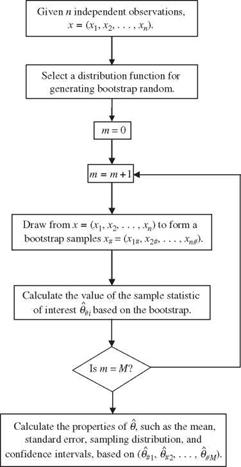
The basic algorithm of the bootstrap technique in estimating the standard deviation associated with any statistic of interest from a set of sample observa­tions involves the following steps:

1. For a set of sample observations of size n, that is, x = {x1, x2,…, xn}, as­sign a probability mass 1/n to each observation according to an empirical probability distribution f,

f: P (X = xi) = 1/n for i = 1,2,…, n (6.111)

2. Randomly draw n observations from the original sample set using f to form a bootstrap sample x# = {x1#, x2#,…, xn#}. Note that the bootstrap sample x# is a subset of the original samples x.

3. Calculate the value of the sample statistic ©# of interest based on the boot­strap sample x #.

4. Independently repeat steps 2 and 3 a number of times M, obtaining bootstrap replications of в# = {в #1, в#2,…, B#M}, and calculate

Resampling Techniques

(6.112)


=


Resampling Techniques

where в#. is the average of the bootstrap replications of ©, that is,

M

в# =Y. в#m/M (6.113)

m=1

A flowchart for the basic bootstrap algorithm is shown in Fig. 6.15. The boot­strap algorithm described provides more information than just computing the

Подпись: Figure 6.15 Flowchart of basic bootstrap resampling algorithm.
Resampling Techniques

standard deviation of a sample statistic. The histogram constructed on the basis of M bootstrap replications 0# = {0#i, 0#2,…, в#м} gives some ideas about the sampling distribution of the sample statistic ©, such as the failure probability. Furthermore, based on the bootstrap replications 0#, one can construct con­fidence intervals for the sample statistic of interest. Similar to Monte Carlo simulation, the accuracy of estimation increases as the number of bootstrap samples gets larger. However, a tradeoff exists between computational cost and the level of accuracy desired. Efron (1982) suggested that M = 200 is generally sufficient for estimating the standard errors of the sample statistics. However, to estimate the confidence interval with reasonable accuracy, one would need at least M = 1000.

This algorithm is called nonparametric, unbalanced bootstrapping. Its para­metric version can be made by replacing the nonparametric estimator f by a

parametric distribution in which the distribution parameters are estimated by the maximum-likelihood method. More specifically, if one judges that on the basis of the original data set the random observations x = (x1, x2,…, xn} are from, say, a lognormal distribution, then the resampling of x’s from x using the parametric mechanism would assume that f is a lognormal distribution.

Note that the theory of the unbalanced bootstrap algorithm just described only ensures that the expected number to be resampled for each individual ob­servation is equal to the number of bootstrap samples M generated. To improve the estimation accuracy associated with a statistical estimator of interest, Davi­son et al. (1986) proposed balanced bootstrap simulation, in which the number of appearances of each individual observation in the bootstrap data set must be exactly equal to the total number of bootstrap replications generated. This constrained bootstrap simulation has been found, in both theory and practical implementations, to be more efficient than the unbalanced algorithm in that the standard error associated with © by the balanced algorithm is smaller. This implies that fewer bootstrap replications are needed by the balanced algorithm than the unbalanced approach to achieve the same accuracy level in estima­tion. Gleason (1988) discussed several computer algorithms for implementing the balanced bootstrap simulation.

Example 6.15 Based on the annual maximum flood data listed in Table 6.4 for Miller Creek, Los Molinos, California, use the unbalanced bootstrap method to estimate the mean, standard errors, and 95 percent confidence interval associated with the annual probability that the flood magnitude exceeds 20,000 ft3/s.

Solution In this example, M = 2000 bootstrap replications of size n = 30 from {yi = ln(Xi)}, i = 1, 2,…, 30, are generated by the unbalanced nonparametric boot­strap procedure. In each replication, the bootstrapped flows are treated as lognormal

TABLE 6.4 Annual Maximum Floods for Mill Creek near Los Molinos, California

Year

Discharge (ft3/s)

Year

Discharge (ft3/s)

1929

1,500

1944

3,220

1930

6,000

1945

3,230

1931

1,500

1946

6,180

1932

5,440

1947

4,070

1933

1,080

1948

7,320

1934

2,630

1949

3,870

1935

4,010

1950

4,430

1936

4,380

1951

3,870

1937

3,310

1952

5,280

1938

23,000

1953

7,710

1939

1,260

9154

4,910

1940

11,400

1955

2,480

1941

12,200

1956

9,180

1942

11,000

1957

6,140

1943

6,970

1958

6,880

Resampling Techniques

variates based on which the exceedance probability P(Q > 20,000 ft3/s) is computed. The results of the computations are shown below:

Statistic

P(Q > 20,000 ft3/s)

Mean

0.0143

Coefficient of variation

0.829

Skewness coefficient

0.900

95 percent confidence interval

(0.000719, 0.03722)

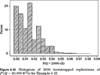
The histogram of bootstrapped replications of P (Q > 20,000 ft3/s) is shown in Fig. 6.16.

Note that the sampling distribution of the exceedance probability P (Q > 20,000 ft3/s) is highly skewed to the right. Because the exceedance probability has to be bounded between 0 and 1, density functions such that the beta distribution may be applicable. The 95 percent confidence interval shown in the table is obtained by truncating 2.5 percent from both ends of the

Control-variate method

The basic idea behind the control-variate method for variance reduction is to take advantage of the available information for the selected variables related to the quantity to be estimated. Referring to Eq. (6.91), the quantity G to be estimated is the expected value of the output of the model g(X). The value of G can be estimated directly by those techniques described in Sec. 6.6. However, a reduction in estimation error can be achieved by indirectly estimating the mean of a surrogate model g(X, Z) as (Ang and Tang, 1984)

g(X, Z) = g(X) – Z(g'(X) – E[g'(X)]} (6.100)

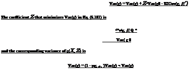
Подпись: Var(g) = Var(g) + Z2Var(g0 - 2ZCov(g, g') The coefficient Z that minimizes Var(g) in Eq. (6.101) is C°v(g, g Q * Var( g 0 and the corresponding variance of g(X, Z) is Var(g) = (1 - pg, g, )Var(g) < Var(g) Control-variate method

in which g'(X) is a control variable with the known expected value E[g'(X)], and Z is a coefficient to be determined in such a way that the variance of g(X, Z) is minimized. The control variable g'(X) is also a model, which is a function of the same stochastic variables X as in the model g(X). It can be shown that g(X, Z) is an unbiased estimator of the random model output g(X), that is, E[g(X, Z)] = E[g(X)] = G. The variance of g(X, Z), for any given Z, can be obtained as

in which pg, gі is the correlation coefficient between the model output g(X) and the control variable g'(X). Since both model output g(X) and the control vari­able g ‘(X) depend on the same stochastic variables X, correlation to a certain degree exists between g(X) and g'(X). As can be seen from Eq. (6.103), using a control variable g ‘(X) could result in a variance reduction in estimating the expected model output. The degree of variance reduction depends on how large the value of the correlation coefficient is. There exists a tradeoff here. To attain a high variance reduction, a high correlation coefficient is required, which can be achieved by making the control variable g'(X) a good approximation to the model g(X). However, this could result in a complex control variable for which the expected value may not be derived easily. On the other hand, the use of a simple control variable g'(X) that is a poor approximation of g(X) would not result in an effective variance reduction in estimation.

The attainment of variance reduction, however, cannot be achieved from total ignorance. Equation (6.103) indicates that variance reduction for estimating G is possible only through the correlation between g(X) and g'(X). However, the correlation between g(X) and g'(X) is generally not known in real-life situa­tions. Consequently, a sequence of random variates of X must be produced to compute the corresponding values of the model output g(X) and the control variable g'(X) to estimate the optimal value of Z* by Eq. (6.102). The general algorithm of the control-variate method can be stated as follows.

1. Select a control variable g'(X).

2. Generate random variates for X(i) according to their probabilistic laws.

3. Compute the corresponding values of the model g(X(i)) and the control vari­able g’ (X(i)).

4. Repeat steps 2 and 3 n times.

5. Estimate the value Z*, according to Eq. (6.102), by

Подпись: (6.104) (6.105) c En=1(g(° – g)[g/(° – E(gQ]

* n Var(g 0

Z ЕП=1і£(0 – g]fe'(0 – E(g0]

Z* En=1k'(0 – E (g OP

depending on whether the variance of the control variable g ‘(X) is known or not.

6. Estimate the value of G, according to Eq. (6.100), by

Подпись: (6.106)G = -]T (g(i) – Z* g/(i)) + Z* e (g о

i=1

Further improvement in accuracy could be made in step 2 of this above algo­rithm by using the antithetic-variate approach to generate random variates.

This idea of the control-variate method can be extended to consider a set of J control variates g'(X) = [g(X), g2(X), …, gJ(X)]г. Then Eq. (6.100) can be modified as

J

g (X, Z) = g (X) -£ Zj {g j (X) – E[g j (X)]} (6.107)

j=1

The vector of optimal coefficients Z*= (Z*nZ*2,… ,Z* J ) that minimizes the vari­ance of g(X, Z) is

in which c is a J x 1 cross-covariance vector between J control variates g'(X) and the model g(X), that is, c = {Cov[g(X),g[(X)],Cov[g(X),g’2(X)], Cov[g(X), g J (X)]}, and C is the covariance matrix of the J control variates, that is, C = [oij] = [ g i (X), g j (X)], for i, j = 1,2,…, J. The corresponding minimum variance of the estimator g(X, Z) is

Var(g) = Var(g) – ctCc= (1 – pgg,) Var(g) (6.109)

in which pg, gі is the multiple correlation coefficient between g(X) and the vector of control variates g'(X). The squared multiple correlation coefficient is called the coefficient of determination and represents the percentage of variation in the model outputs g(X) explained by the J control variates g'(X).

Latin hypercube sampling technique

The Latin hypercube sampling (LHS) technique is a special method under the umbrella of stratified sampling that selects random samples of each random variable over its range in a stratified manner. Consider a multiple integral involving K random variables

G = g (x) fx (x) d x = E [g (X)] (6.91)

J xeE

where X = (X1, X 2,…, XK )t is an K-dimensional vector of random variables, and fx(x) is their joint PDF.

The LHS technique divides the plausible range of each random variable into M(M > K in practice) equal-probability intervals. Within each interval, a single random variate is generated resulting in M random variates for each random variable. The expected value of g(X), then, is estimated as

1 M

G = g( X 1m, X 2m, …, XKm ) (6.92)

m=1

where Xkm is the variate generated for the kth random variable Xk in the mth set.

More specifically, consider a random variable Xk over the interval of [xk, xk ] following a specified PDF fk(xk). The range [xk, xk] is partitioned into M inter­vals, that is,

xk — xk0 < xk1 < xk2 < ”’ < xk, M—1 < xkM — xk (6.93)

in which P (xkm < Xk < xk, m+1) = 1/M for all m = 0, 1, 2,…, M — 1. The end points of the intervals are determined by solving

/

xkm m

fk (xk) dxk = m (6.94)

-k

where Fk ( ) is the CDF of the random variable Xk. The LHS technique, once the end points for all intervals are determined, randomly selects a single value

in each of the intervals to form the M samples set for Xk. The sample values can be obtained by the CDF-inverse or other appropriate method.

To generate M values of random variable Xk from each of the intervals, a sequence of probability values {pk1, pk2,…, pk, M-1, pkM} is generated as

m — 1

Pkm = M + Zkm m = 1,2,…, M (6.95)

in which {zk1, Zk2,…, Zk, M-1, ZkM} are independent uniform random numbers from Z ~ U(0, 1/M). After {pk1, pk2,…, pk, M-1, pkM} are generated, the corre­sponding M random samples for Xk can be determined as

Xkm = F-l( pkm) m = 1,2,…, M (6.96)

Note that pkm determined by Eq. (6.96) follows

pk1 < pk2 < ••• < pkm < ••• < pk, M-1 < pkM (6.97)

and accordingly,

xk1 — xk2 — — xkm — ‘ — xk, M-1 — xkM (6.98)

To make the generated {xk1, xk2,…, xk, M-1, xkM} a random sequence, random permutation can be applied to randomize the sequence. Alternatively, Latin hypercube samples for K random variables with size M can be generated by (Pebesma and Heuvelink, 1999), that is,

xkm = Fj-1^Skm MUkm ) (6.99)

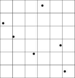
where skm is a random permutation of 1 to M, and ukm is a uniformly distributed random variate in [0, 1]. Figure 6.14 shows the allocation of six samples by the LHS technique for a problem involving two random variables. It is seen that in each row or column of the 6 x 6 matrix only one cell contains a generated sample. The LHS algorithm can implemented as follows:

1. Select the number of subintervals M for each random variable, and divide the plausible range into M equal-probability intervals according to Eq. (6.94).

2. Generate M standard uniform random variates from U(0, 1/M).

3. Determine a sequence of probability values pkm, for k = 1, 2,…, K; m = 1,2,…, M, using Eq. (6.95).

4. Generate random variates for each of the random variables using an appro­priate method, such as Eq. (6.96).

5. Randomly permutate generated random sequences for all random variables.

6. Estimate G by Eq. (6.92).

Using the LHS technique, the usual estimators of G and its distribution function are unbiased (McKay, 1988). Moreover, when the function g(X) is

x21 x20

Подпись:Подпись: x24Подпись: X2 X23Подпись: x22Подпись:Latin hypercube sampling techniquemonotonic in each of the Xk, the variances of the estimators are no more than and often less than the variances when random variables are generated from simple random sampling. McKay (1988) suggested that the use of twice the number of involved random variables for sample size (M > 2K) would be suf­ficient to yield accurate estimation of the statistics model output. Iman and Helton (1985) indicated that a choice of M equal to 4/3K usually gives satisfac­tory results. For a dynamic stream water-quality model over a 1-year simula­tion period, Manache (2001) compared results from LHS using M = 4/3K and M = 3K and found reasonable convergence in the identification of the most sensitive parameters but not in calculation of the standard deviation of model output. Thus, if it is computationally feasible, the generation of a larger num­ber of samples would further enhance the accuracy of the estimation. Like all other variance-reduction Monte Carlo techniques, LHS generally would require fewer samples or model evaluations to achieve an accuracy level comparable with that obtained from a simple random sampling scheme. In hydrosystems engineering, the LHS technique has been applied widely to sediment transport (Yeh and Tung, 1993; Chang et al., 1993), water-quality modeling (Jaffe and Ferrara, 1984; Melching and Bauwens, 2001; Sohrabi et al., 2003; Manache and Melching, 2004), and rainfall-runoff modeling (Melching, 1995; Yu et al., 2001; Christiaens and Feyen, 2002; Lu and Tung, 2003).
Melching (1995) compared the results from LHS with M = 50 with those from Monte Carlo simulation with 10,000 simulations and also with those from FOVE and Rosenbleuth’s method for the case of using HEC-1 (U. S. Army Corps

of Engineers, 1991) to estimate flood peaks for a watershed in Illinois. All meth­ods yielded similar estimates of the mean value of the predicted peak flow. The variation of standard deviation estimates among the methods was much greater than that of the mean value estimates. In the estimation of the standard devia­tion of the peak flow, LHS was found to provide the closest agreement to Monte Carlo simulation, with an average error of 7.5 percent and 10 of 16 standard deviations within 10 percent of the value estimated with Monte Carlo simu­lation. This indicates that LHS can yield relatively accurate estimates of the mean and standard deviation of model output at a far smaller computational burden than Monte Carlo simulation. A detailed description of LHS, in con­junction with the regression analysis for uncertainty and sensitivity analysis, can be found elsewhere (Tung and Yen, 2005, Sec. 6.8).

Example 6.14 Referring to Example 6.7, apply the Latin hypercube sampling tech­nique to evaluate the pump failure probability in the time interval [0, 200 h].

Solution Again, the uniform distribution U(0, 200) is selected along with the sample- mean Monte Carlo method for carrying out the integration. In Latin hypercube sam­pling, the interval [0, 200] is divided into 1000 equal-probability subintervals, with each having a probability of 0.001. For U(0, 200), the end points of each subinterval can be obtained easily as

t0 = 0 t1 = °-2, t2 = °-4, ■ ■■ , £999 = 199.8, t1000 = 200

By the LHS, one random variate for each subinterval is generated. In other words, generate a single random variate from

Um ~ U[0.2(m — 1), 0.2m] m = 1, 2,…, 1000

The algorithm for estimating the pump failure probability involves the following steps:

1. Initialize the subinterval index m = 0.

2. Let m = m + 1. Generate one standard uniform random variate um, and transform

it into the random variate from the corresponding subinterval by tm = 0.2(m — 1) +

um.

3. If m < 1000, go to step 2; otherwise, compute the pump failure probability as

1 1000

pf = 1000 £ ft(tm)

m=1

and the associated standard deviation as

__ sm

Spf = V1000

with sm representing the standard deviation of 1000 computed function values

ft ™.

The results from the numerical simulation are

The 95 percent confidence interval is (0.14743, 0.14828). The value of pf is extremely close to the exact solution of 0.147856, and only 1000 simulations were used.

Stratified sampling technique

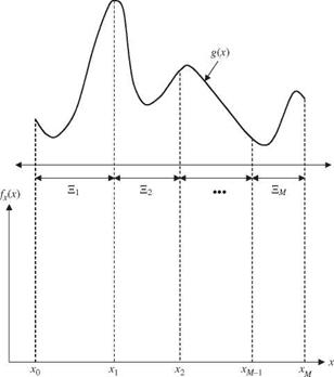
The stratified sampling technique is a well-established area in statistical sam­pling (Cochran, 1966). Variance reduction by the stratified sampling technique is achieved by taking more samples in important subregions. Consider a prob­lem in which the expectation of a function g (X) is sought, where X is a random variable with a PDF fx(x), x є E. Referring to Fig. 6.13, the domain E for the random variable X is divided into M disjoint subregions Em, m = 1, 2,…, M. That is,

m

S = U Sm 0 = Sm Fl Sm! m = m

m=1

Stratified sampling technique

Let pm be the probability that random variable X will fall within the sub­region Em, that is, f fx(x)dx = pm. Therefore, it is true that Lmpm = 1.

The expectation of g (X) can be computed as

m.. M

G = g(x) fx(x) dx =^2 / g(x) fx(x) dx =^2 Gm (6.86)

m=1J Em m=1

where Gm = fw g (x) fx(x) dx.

Note that the integral for Gm can be written as

Stratified sampling technique

(6.87)


(6.88)


Stratified sampling technique

Подпись: M G =Y, G m m=l Stratified sampling technique Подпись: nm Eg( Xmi) _i = 1 Подпись: (6.89)

where nm is the number of sample points in the mth subregion, and Lmnm = n, the total number of random variates to be generated. Therefore, the estimator for G in Eq. (6.86) can be obtained as

After the number of subregions M and the total number of samples n are determined, an interesting issue for the stratified sampling is how to allo­cate the total n sample points among the M subregions such that the variance associated with G by Eq. (6.89) is minimized. A theorem shows that the optimal n*m that minimizes Var(G) in Eq. (6.89) is (Rubinstein, 1981)

Подпись: (6.90)Подпись: nm=npm&m

v^M p _

Xm’ = 1 P m’ °m!

where am is the standard deviation associated with the estimator Gm in Eq. (6.88).

In general, information about am is not available in advance. It is suggested that a pilot simulation study be made to obtain a rough estimation about the value of am, which serves as the basis in the follow-up simulation investigation to achieve the variance-reduction objective.

A simple plan for sample allocation is nm = npm after the subregions are specified. It can be shown that with this sampling plan, the variance associated with G by Eq. (6.89) is less than that from the simple random-sample technique. One efficient stratified sampling technique is systematic sampling (McGrath, 1970), in which pm = 1/M and nm = n/M. The algorithm of the systematic sampling can be described as follows:

1. Divide interval [0, 1] into M equal subintervals.

2. Within each subinterval, generate n/M uniform random numbers umi ~ U[(m — 1)/n, m/n], m = 1, 2,…, M; i = 1, 2,…, n/m.

3. Compute Xmi = F—l(Umi).

4. Calculate G according to Eq. (6.89).

Example 6.13 Referring to Example 6.7, apply the systematic sampling technique to evaluate the pump failure probability in the time interval [0, 200 h].

Solution Again, let us adopt the uniform distribution U(0, 200) and carry out the computation by the sample-mean Monte Carlo method. In the systematic sampling, the interval [0, 200] is divided into 10 equal-probability subintervals, each having a probability content of 0.1. Since h(t) = 1/200, 0 < t < 200, the end points of each subinterval can be obtained easily as

tQ = 0, t1 = 20, t2 = 40,…, t9 = 180, t10 = 200

Furthermore, let us generate nm = 200 random variates from each subinterval so that £mnm = 2000. This can be achieved by letting

20(m — 1) 20m 10 , "00”


U


for i = 1, 2,…, 200; m = 1, 2,… ,10


U„


The algorithm for estimating the pump failure probability is the following:

1. Initialize subinterval index m = 0.

2. Let m = m + 1. Generate nm = 200 standard uniform random variates {um1, um2,…, um,200}, and transform them into the random variates from the corre­sponding subinterval by tmi = 20(m — 1) + 20umi, for i = 1, 2,…, 200.

3. Compute pf, m as

Подпись: 200

pf, m = 200 5-/ ft(tmi)

mi = 1

and the associated variance as

Подпись: Var( p f ,m) =p2 s2 0 12s2

m m. m

nm 200

in which sm is the standard deviation of 200 ft(tmi) for the mth subinterval.

4. If m < 10, go to step 2; otherwise, compute the pump failure probability as

1 10

P f = 10 E p f m

m=1

and the associated standard error as

“I 1/2


10


1


m=1

The results from the numerical simulation are shown below:

m

p f, m

sm

m

p f, m

sm

1

0.15873

0.00071102

6

0.14659

0.00066053

2

0.15626

0.00069358

7

0.14423

0.00064361

3

0.15374

0.00069298

8

0.14194

0.00064993

4

0.15121

0.00072408

9

0.13968

0.00066746

5

0.14887

0.00065434

10

0.13742

0.00067482

All 0.14787

0.15154 x 10—5

The value of pf is extremely close to the exact solution of 0.147856.

Correlated-sampling techniques

Correlated-sampling techniques are especially effective for variance reduction when the primary objective of the simulation study is to evaluate small changes in system performance or to compare the difference in system performances between two specific designs (Rubinstein, 1981; Ang and Tang, 1984). Consider that one wishes to estimate

Подпись:Подпись: (6.81)A© = ©1 — ©2

in which

©1 = J g1(x) f 1(x) dx = E [ g1(X)] ©2 = / g2(y) f2(y) dy = E [ g2(Y)]

Подпись: A© = ©1 — ©2 Подпись: 1 n Подпись: Eg1( Xi) — E g2(Yi) . i = 1 i = 1 Correlated-sampling techniques Подпись: (6.82)

with f 1(x) and f 2(y) being two different PDFs. By Monte Carlo simulation, A© can be estimated as

in which Xi andYi are random samples generated from f 1(x) and f2(y), re­spectively, and A©i = g1(Xi) — gjjYi).

The variance associated with A© is

Var(A©) = Var(©©1) + Var(©2) — 2Cov(©b ©2) (6.83)

In the case that random variates Xi and Yi are generated independently in the Monte Carloalgorithm, ©1 and ©2 also would be independent random variables.

Hence Var(A©) = Var((©1) + Var(©2)________________________

Note that from Eq. (6.83), Var(A©) can be reduced if positively corre­lated random variables ©1 and ©2 can be produced to estimate A©. One easy way to obtain positively correlated samples is to use the same sequence of uniform random variates from U(0, 1) in both simulations. That is, the ran­dom sequences {X1, X 2,…, Xn} and {Y1, Y 2,…, Yn} are generated through Xi = F—l(Ui) and Yi = F—1(Ui), respectively.

The correlated-sampling techniques are especially effective in reducing vari­ance when the performance difference between two specific designs for a system involve the same or similar random variables. For example, consider two de­signs A and B for the same system involving a vector of K random variables X = (X1, X2,…, XK), which could be correlated with a joint PDF fx(x) or be independent of each other with a marginal PDF fk(xk), k = 1, 2,…, K. The performance of the system under the two designs can be expressed as

Подпись: OA,I = g &B,i = g Correlated-sampling techniques Подпись: i = 1,2,..., n (6.85a) i = 1, 2,..., n (6.85b)

Подпись: p f, AПодпись: P f, B

Подпись: in which xki = Fk (uki) is the inverse CDF for the kth random variable Xk operating on the kth standard uniform random variate for the ith simulation.
Подпись: Example 6.12 Refer to the pump reliability problem that has been studied in previous examples. Now consider a second pump the time-to-failure PDF of which also is an exponential distribution but has a different parameter of в = 0.0005/h. Estimate the difference in the failure probability between the two pumps over the time interval [0, 200 h] using the correlated-sampling technique with n = 2000. Solution Again, the sample-mean Monte Carlo method with a uniform distribution U(0, 200) is applied as in Example 6.7. In this example, the same set of standard uniform random variates {u1, U2,..., U2000} fromU(0,1) is used to estimate the failure probabilities for the two pumps as
Подпись: — Y (0.0008e-a0008ti i=1
Подпись: — Y (0.0005e-°m°5ti i=1
Подпись: in which ti = 200ui, for i = 1, 2,..., 2000. The difference in failure probabilities can be estimated as
Подпись: Apf = pf,A - Pf,B = 0.05276
Подпись: which is within 0.125 percent of the exact solution e 0 0005(20°) — e о.оооазоо) = e-01 — e—016 = 0.0526936. The standard deviation of the 2000 differences in failure probability Ai = 200[ fA(ti) — fB (ti)], i = 1,2,... ,2000, is 0.00405. Hence the standard error associated with the estimated difference in failure probability is 0.00405/V2000 = 0.00009.

in which g( ) is a function defining the system performance, and a and b are vectors of design parameters corresponding to designs A and B, respectively. Since the two performance measures ©A and ©B are dependent on the same random variables through the same performance function g( ), their estimators will be positively correlated. In this case, independently generating two sets of K random variates, according to their probability laws for designs A and B, still wouldresult in a positive correlation between ©A and ©B. To further reduce Var(A©), an increase in correlation between ©A and ©B can be achieved using a common set of standard uniform random variates for both designs A and B by assuming that system random variables are independent, that is,

For the sake of examining the effectiveness of the correlated-sampling technique, let us separately generate a set of independent standard uniform random variates {Ир u2,…, U2000} and use them in calculating the failure probability for pump B. Then the estimated difference in failure probability between the two pumps is 0.05256, which is slightly larger than that obtained by the correlated-sampling technique. However, the standard error associated with Ai = 200[f a(4) — f в(t)] then is

0. 00016, which is larger than that from the correlated-sampling technique.