Category Hydrosystems Engineering Reliability Assessment and Risk Analysis

Generating multivariate normal random variates

A random vector X = (X1, X2,…, XK)t has a multivariate normal distribution with a mean vector fj, x and covariance matrix Cx, denoted as X ~ N(px, Cx). The joint PDF of K normal random variables is given in Eq. (2.112). To gener­ate high-dimensional multivariate normal random variates with specified (j, x

Generating multivariate normal random variates

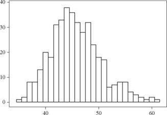
Drawdown recess time (days)

Figure 6.4 Histogram of simulated drawdown recess time for Exam­ple 6.4.

and Cx, the CDF-inverse algorithm described in Sec. 6.5.1 might not be efficient. In this section, two alternative algorithms for generating multivariate normal random variates are described. Both algorithms are based on orthogonal trans­formation using the covariance matrix Cx or correlation matrix Rx described in Sec. 2.7.1. The result of the transformation is a vector of independent nor­mal variables, which can be generated easily by the algorithms described in Sec. 6.4.1.

Square-root method. The square-root algorithm decomposes the covariance ma­trix Cx or correlation matrix R x into

Rx = LLt Cx = L Lt

as shown in Appendix 4B, in which L and L are K x K lower triangular matrices associated with the correlation and covariance matrices, respectively. Accord­ing to Eq. (4B.12), L = DЦ2L, with Dx being the K x K diagonal matrix of variances of the K involved random variables.

In addition to being symmetric, if Rx or Cx is a positive-definite matrix, the Cholesky decomposition (see Appendix 4B) is an efficient method for finding the unique lower triangular matrices L or L (Young and Gregory, 1973; Golub and Van Loan, 1989). Using the matrix L or L, the vector of multivariate normal random variables can be expressed as

X = fix + L Z = fix + D1/2 LZ (6.34)

in which Z’ is an K x 1 column vector of independent standard normal vari­ables. It was shown easily in Appendix 4B that the expectation vector and the covariance matrix of the right-hand side in Eq. (6.34), E(px + L Z’), are equal
to fix and Cx, respectively. Based on Eq. (6.34), the square-root algorithm for

generating multivariate normal random variates can be outlined as follows:

1. Compute the lower triangular matrix associated with the correlation or co­variance matrix by the Cholesky decomposition method.

2. Generate K independent standard normal random variates z’ = (z’x, z’2,…, z’K)t from N(0, 1).

3. Compute the corresponding normal random variates by Eq. (6.34).

4. Repeat steps 1 through 3 to generate the desired number of sets of normal random vectors.

Example 6.5 Refer to Example 6.4. Apply the square-root algorithm to estimate the statistical properties of the drawdown recess time, including its mean, standard deviation, and skewness coefficient. Compare the results with Example 6.4.

Solution By the square-root algorithm, the covariance matrix of permeability Kh and storage coefficient S,

Подпись: 0.012 0.5(0.01)(0.005) 0.0001 0.000025 0.5(0.01)(0.005) 0.0052 0.000025 0.000025 C (Kh, S)

is decomposed into the multiplication of the two lower triangular matrices, by the Cholesky decomposition, as

0. Подпись: L01 0′

0.0025 0.00443

The Monte Carlo simulation can be carried out by the following steps:

1. Generate a pair of standard normal variates z1 and z2.

2. Compute the permeability Kh and storage coefficient S simultaneously as

Generating multivariate normal random variates

0.1

0.05


+


3. Use (kh, s) generated from step 2 in Eq. (6.29) to compute the corresponding draw­down recess time t.

4. Repeat steps 1 through 3 n = 400 times to obtain 400 realizations of drawdown recess times {ti, t2,…, t400}.

5. Compute the mean, standard deviation, and skewness coefficient of the drawdown recess time.

The results from carrying out the numerical simulation are

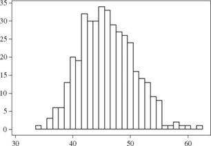
Mean fit = 45.94 days Standard deviation at = 4.69 days Skewness coefficient yt = 0.301

The histogram of400 simulated drawdown recess times is shown in Fig. 6.5. The mean and standard deviation are very close to those obtained in Example 6.4, whereas the

Generating multivariate normal random variates

Drawdown recess time (days)

Figure 6.5 Histogram of simulated drawdown recess time for Example 6.5.

skewness coefficient is 62 percent of that found in Example 6.4. This indicates that 400 simulations are sufficient to estimate the mean and standard deviation accurately, but more simulations are needed to estimate the skewness coefficient accurately.

Spectral decomposition method. The basic idea of spectral decomposition is de­scribed in Appendix 4B. The method finds the eigenvalues and eigenvectors of the correlation or covariance matrix of the multivariate normal random vari­ables. Through the spectral decomposition, the original vector of multivariate normal random variables X, then, is related to a vector of independent standard normal random variables Z’ ~ N(0,1) as

X = + D1/[10] [11] [12] У A1/2 Z’ = ^х + V Л1/2 Z’ (6.36)

in which V and Л are the eigenvector and diagonal eigenvalue matrices of Cx, respectively, whereas V and Л are the eigenvector and diagonal eigen­value matrices of Rx, respectively. Equation (6.36) clearly reveals the necessary computations for generating multivariate normal random vectors. The spectral decomposition algorithm for generating multivariate normal random variates involves the following steps:

Many efficient algorithms have been developed to determine the eigenvalues and eigenvectors of a symmetric matrix. For the details of such techniques, readers are referred to Golub and Van Loan (1989) and Press et al. (1992).

Generation of Vectors of Multivariate Random Variables

In preceding sections, discussions focused on generating univariate random variates. It is not uncommon for hydrosystems engineering problems to involve multiple random variables that are correlated and statistically dependent. For example, many data show that the peak discharge and volume of a runoff hy­drograph are positively correlated. To simulate systems involving correlated random variables, generated random variates must preserve the probabilis­tic characteristics of the variables and the correlation structure among them. Although multivariate random number generation is an extension of the uni­variate case, mathematical difficulty and complexity associated with multi­variate problems increase rapidly as the dimension of the problem gets larger.

Compared with generating univariate random variates, multivariate random variate generation is much more restricted to fewer joint distributions, such as multivariate normal, multivariate lognormal, and multivariate gamma (Ronning, 1977; Johnson, 1987; Parrish, 1990). Nevertheless, the algorithms for generating univariate random variates serve as the foundation for many multivariate Monte Carlo algorithms.

6.5.1 CDF-inverse method

This method is an extension of the univariate case described in Sec. 6.3.1. Con­sider a vector of K random variables X = (X1, X 2,…, XK ) having a joint PDF of

f x (x) = f 1,2,…, K (X1, X2, … , XK ) (6.23)

This joint PDF can be decomposed to

fx(x) = f 1(X1) X f2(X2X1) X—X fK(XK|X1,X2, …,XK-1) (6.24)

in which f 1(x1) and fk(xk |x1, x2, …, xk-1) are, respectively, the marginal PDF and the conditional PDF of random variables X1 and Xk. In the case when all K random variables are statistically independent, Eq. (6.23) is simplified to

K

fx(x) = fk (Xk) (6.25)

k=1

One observes that from Eq. (6.25) the joint PDF of several independent random variables is simply the product of the marginal PDF of the individual random variable. Therefore, generation of a vector of independent random variables can be accomplished by treating each individual random variable separately, as in the case of the univariate problem. However, treatment of random variables cannot be made separately in the case when they are correlated. Under such circumstances, as can be seen from Eq. (6.24), the joint PDF is the product of conditional distributions. Referring to Eq. (6.24), generation of K random variates following the prescribed joint PDF can proceed as follows:

1. Generate random variates for X1 from its marginal PDF f 1(x1).

2. Given X1 = x1 obtained from step 1, generate X2 from the conditional PDF f 2(X2 |X1).

3. With X1 = X1 and X2 = X2 obtained from steps 1 and 2, produce X3 based on f 3(X3|X1, X2).

4. Repeat the procedure until all K random variables are generated.

To generate multivariate random variates by the CDF-inverse method, it is required that the analytical relationship between the value of the variate

and the conditional distribution function is available. Following Eq. (6.24), the product relationship also holds in terms of CDFs as

Fx(x) = Fi(xi) X FiteXi) X—X Fk(XK|xi, X2,…, xk-i) (6.26)

in which Fi(xi) and Fk(xk|xi, x2,…,xk-i) are the marginal CDF and condi­tional CDF of random variables Xi and Xk, respectively. Based on Eq. (6.26), the algorithm using the CDF-inverse method to generate n sets of K multi­variate random variates from a specified joint distribution is described below (Rosenblatt, i952):

1. Generate K standard uniform random variates uiy u2,…, uK from U(0, i).

2. Compute

= F-i(ui = F2ri(u2 |xi)

xk = F-1(uu |xi, x2,…., xk-i)

3. Repeat steps i and 2 for n sets of random vectors.

There are K! ways to implement this algorithm in which different orders of random variates Xk, k = i, 2,…, K, are taken to form the random vector X. In general, the order adopted could affect the efficiency of the algorithm.

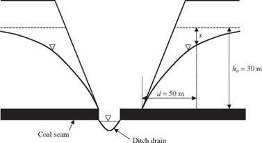
Example 6.4 This example is extracted from Nguyen and Chowdhury (i985). Con­sider a box cut of an open strip coal mine, as shown in Fig. 6.3. The overburden has a phreatic aquifer overlying the coal seam. In the next bench of operation, excavation is to be made 50 m (d = 50 m) behind the box-cut high wall. It is suggested that for

Generation of Vectors of Multivariate Random Variables

Figure 6.3 Box cut of an open strip coal mine resulting in water drawdown. (After Nguyen and Chowdhury, 1985.)

safety reasons of preventing slope instability the excavation should start at the time when the drawdown in the overburden d = 50 m away from the excavation point has reached at least 50 percent of the total aquifer depth (ho).

Generation of Vectors of Multivariate Random Variables

Nguyen and Raudkivi (1983) gave the transient drawdown equation for this prob­lem as

Generation of Vectors of Multivariate Random Variables
Подпись: 1
Подпись: (s - Us) - Pkh,s(ffs/ffkh)(kh - Mkh)

(6.31)

From the conditional PDF given earlier, the conditional expectation and conditional standard deviation of storage coefficient S, given a specified value of permeability Kh = kh, can be derived, respectively, according to Eqs. (2.110) and (2.111), as

ffs

MSkh = E(SKh = kh) = Ms + Pkh, s—— (kh – Mkh) (6.32)

ffkh

ffskh = ffsy 1 – plh s (6.33)

Therefore, the algorithm for generating bivariate normal random variates to esti­mate the statistical properties of the drawdown recess time can be outlined as follows:

1. Generate a pair of independent standard normal variates and z’2.

2. Compute the corresponding value of permeability kh = Mkh + ^khZy

3. Based on the value of permeability obtained in step 2, compute the conditional mean and conditional standard deviation of the storage coefficient according to Eqs. (6.32) and (6.33), respectively. Then calculate the corresponding storage coef­ficient as S = Mskh + ffskhZ2.

4. Use Kh = kh and S = s generated in steps 3 and 4 in Eq. (6.29) to compute the corresponding drawdown recess time t.

5. Repeat steps 1 through 4 n = 400 times to obtain 400 realizations of drawdown recess times {t1, t2,…, t400}.

6. Compute the sample mean, standard deviation, and skewness coefficient of the drawdown recess time according to the last column of Table 2.1.

The histogram ofthe drawdown recess time resulting from 400 simulations is shown in Fig. 6.4. The statistical properties of the drawdown recess time are estimated as

Mean nt = 45.73 days

Standard deviation at = 4.72 days

Skewness coefficient yt = 0.487

Other univariate distributions and computer programs

The algorithms described in the preceding subsections are for some probability distributions commonly used in hydrosystems engineering and analysis. One might encounter other types of probability distributions in an analysis that are not described herein. There are several books that have been written for gen­erating univariate random numbers (Rubinstein, 1981; Dagpunar, 1988; Gould and Tobochnik, 1988; Law and Kelton, 1991). To facilitate the implementa­tion of Monte Carlo simulation, computer subroutines in different languages are available (Press et al., 1989, 1992, 2002; IMSL, 1980). In addition, many other spreadsheet-based computer software, such as Microsoft Excel, @Risk, and Crystal Ball, contain statistical functions allowing the generation of ran­dom variates of various distributions.

Poisson distribution

The Poisson random variable is discrete, having a PMF fx(xi) = P (X = xi) given in Eq. (2.53). Dagpunar (1988) presented a simple algorithm and used the CDF-inverse method based on Eq. (6.7). When generating Poisson ran­dom variates, care should be taken so that e~v is not smaller than the ma­chine’s smallest positive real value. This could occur especially when the Poisson

parameter v is large. An algorithm for generating Poisson random variates is as follows:

1. Generate u ~ U(0,1) and initialize x = 0 and y = e~v

2. If y < u, go to step 3. Otherwise, x is the Poisson random variate sought.

3. Let u = u – y, x = x + 1, and update y = vy/x. Then go to step 2.

This algorithm is efficient when v < 20. For a large v, the Poisson distribution can be approximated by a normal distribution with a mean v — 0.5 and standard deviation of>. Then a Poisson random variate is set to the round-off normal random variate from N(v — 0.5^/v).

Other algorithms have been developed for generating Poisson random vari­ates. Rubinstein (1981) used the fact that the interarrival time between events for a Poisson process has an exponential distribution with parameter 1/v. Atkinson (1979) applied the AR method using a logistic distribution as the enveloping PDF.

Gamma distribution

The gamma distribution is used frequently in the statistical analysis of hydro­logic data. For example, Pearson type III and log-Pearson type III distributions used in the flood frequency analysis are members of the gamma distribution family. It is a very versatile distribution the PDF of which can take many forms (see Fig. 2.20). The PDF of a two-parameter gamma random variable, denoted by X ~ GAM(a, в), is given by Eq. (2.72). The standard gamma PDF involving one-parameter a can be derived using variable transformation by letting

Y = X/в. The PDF of the standard gamma random variable Y, denoted by

Y ~ GAM(a), is shown in Eq. (2.78). The standard gamma distribution is used in all algorithms to generate gamma random variate Y s from which random variates from a two-parameter gamma distribution are obtained from X = вY.

The simplest case in generating gamma random variates is when the shape parameter a is a positive integer (Erlang distribution). In such a case, the random variable Y ~ GAM(a) is a sum of a independent and identical standard exponential random variables with parameter в = 1. The random variates from

Y ~ GAM(a), then, can be obtained as

a

Y = £- ln(U) (6.21)

i = 1

To avoid large numbers oflogarithmic evaluations (when a is large), Eq. (6.21) alternatively can be expressed as

Y = -1п^П Uij (6.22)

Although simplicity is the idea, this algorithm for generating gamma random variates has three disadvantages: (1) It is only applicable to integer-valued shape parameter a, (2) the algorithm becomes extremely slow when a is large, and (3) for a large a, numerical underflow on a computer could occur.

Several algorithms have been developed for generating standard gamma ran­dom variates for a real-valued a. The algorithms can be classified into those which are applicable for the full range (a > 0), 0 < a < 1, and a > 1. Dagpunar (1988) showed that through a numerical experiment, algorithms developed for a full range of a are not efficient in comparison with those especially tailored for subregions. The two efficient AR-based algorithms are presented in Dagpunar (1988).

Lognormal distribution

Consider a random variable X having a lognormal distribution with a mean H-x and standard deviation ox, that is, X ~ LN(^x, ox). For a lognormal random variable X, its logarithmic transform Y = ln(X) leads to a normal distribution for Y. The PDF of X is given in Eq. (2.65). In the log-transformed space, the mean and standard deviation of ln(X) can be computed, in terms of цx and ox, by Eqs. (2.67a) and (2.67b). Since Y = ln(X) is normally distributed, the generation of lognormal random variates from X ~ LN(^x, ox) can be obtained by the following steps:

1. Calculate the mean ^ln x and standard deviation oin x of log-transformed vari­able ln(X) by Eqs. (2.67a) and (2.67b), respectively.

2. Generate the standard normal variate г from N(0,1).

3. Compute y = ,u. lnx + olnxZ.

4. Compute the lognormal random variate x = ey.

6.1.3 Exponential distribution

The exponential distribution is used frequently in reliability computation in the framework of time-to-failure analysis. It is often used to describe the stochastic behavior of time to failure and time-to-repair of a system or component. A ran­dom variable X having an exponential distribution with parameter в, denoted by X ~ EXP(e), is described by Eq. (2.79). By the CDF-inverse method,

u = Fx (x) = 1 – e-x/e (6.18)

so that

Подпись: (6.19)X = – в ln( 1 – U)

Since 1 – U is distributed in the same way as U, Eq. (6.19) is reduced to

X = – в ln(U) (6.20)

Equation (6.20) is also valid for random variables with the standard exponential distribution, that is, V ~ exp(e = 1). The algorithm for generating exponential variates is

1. Generate uniform random variate u from U(0,1).

2. Compute the standard exponential random variate v = – ln(u).

3. Calculate x = vft.

Generation of Univariate Random Numbers for Some Distributions

This section briefly outlines efficient algorithms for generating random variates for some probability distributions commonly used in hydrosystems engineering and analysis.

6.1.2 Normal distribution

A normal random variable with a mean цx and standard deviation ox, denoted as X ~ N(p. x, ox), has a PDF given in Eq. (2.58). The relationship between X and the standardized normal variable Z is

X = ^x + OxZ (6.11)

in which Z is the standard normal random variable having a mean 0 and unit standard deviation, denoted as Z ~ N(0,1). Based on Eq. (6.11), normal ran­dom variates with a specified mean and standard deviation can be generated from standard normal variates. Herein, three simple algorithms for generating standard normal variates are described.

Box-Muller algorithm. The algorithm (Box and Muller, 1958) produces a pair of independent N(0,1) variates as

z1 = v/-2ln(u1) cos(2n u2)

______________ (6.12)

Z2 = /-2ln(U2) sin(2nU2)

in which u1 and u2 are independent uniform variates from U(0,1). The algo­rithm involves the following steps:

1. Generate two independent uniform random variates u1 and u2 from U(0, 1).

2. Compute z1 and z2 simultaneously using u1 and u2 according to Eq. (6.12).

Marsagalia-Bray algorithm. Marsagalia and Bray (1964) proposed an alternative algorithm that avoids using trigonometric evaluations. In their algorithm, two independent uniform random variates u1 and u2 are produced to evaluate the following three expressions:

V1 = 2U1 – 1

V2 = 2U2 – 1 (6.13)

R = V1 + V 22

If R > 1, the pair (u1, u2) is rejected from further consideration, and a new pair (u1, u2) is generated. For the accepted pair, the corresponding standard

Подпись: Zi = V і Подпись: -2ln( R) R Подпись: Z2 = V 2 Подпись: -2ln( R) R Подпись: (6.14)

Подпись: (6.15) (6.16) Подпись:

Подпись: The Marsagalia-Bray algorithm involves the following steps: 1. Generate two independent uniform random variates u1 and u2 from U(0, 1). 2. Compute V1, V2, and R according to Eq. (6.13). 3. Check if R < 1. If it is true, compute the two corresponding N(0, 1) variates using Eq. (6.14). Otherwise, reject (u1, u2) and return to step 1. Algorithm based on the central limit theorem. This algorithm is based on the central limit theorem, which states that the sum ofindependent random variables approaches a normal distribution as the number ofrandom variables increases. Specifically, consider the sum of J independent standard uniform random variates from U(0, 1). The following relationships are true:
Подпись: *( £J V" feUj)=J
Подпись: By the central limit theorem, this sum of J independent U’s would approach a normal distribution with the mean and variance given in Eqs. (6.15) and (6.16), respectively. Constrained by the unit variance of the standard normal variates, Eq. (6.16) yields J = 12. Then a standard normal variate is generated by
Подпись: (6.17)
Подпись: j=1
Подпись: The central limit theorem-based algorithm can be implemented as 1. Generate 12 uniform random variates from U(0, 1). 2. Compute the corresponding standard normal variate by Eq. (6.17). There are many other efficient algorithms developed for generating normal random variates using the variable transformation method and AR method. For these algorithms readers are referred to Rubinstein (1981).

normal variates are computed by

Variable transformation method

The variable transformation method generates a random variate of interest based on its known statistical relationship with other random variables the variates of which can be produced easily. For example, one is interested in generating chi-square random variates with n degrees of freedom. The CDF – inverse method is not appropriate in this case because the chi-square CDF is not analytically expressible. However, knowing the fact that the sum of n squared independent standard normal random variables gives a chi-square random variable with n degrees of freedom (see Sec. 2.6.6), one could generate chi-square random variates from first producing n standard normal random variates, then squaring them, and finally adding them together. Therefore, the variable transformation method is sometimes effective for generating random variates from a complicated distribution based on variates produced from sim­ple distributions. In fact, many algorithms described in the next section are based on the idea of variable transformation.

Acceptance-rejection methods

Consider a problem for which random variates are to be generated from a specified probability density function (PDF) fx(x). The basic idea of the

TABLE 6.3 List of Distributions the Cumulative Distribution Function (CDF) Inverses of which Are Analytically Expressible

Distribution

Fx (x) =

x = Fx fiu)

Exponential

1 — exp(-вx), x > 0

—в ln(1 — F)

Uniform

(x — a)/(b — a)

a + ( b – a) F

Gumbel

exp{ exp[ (x — %)/в)]}

% — в ln[ ln(F)]

Weibull

1 — exp{—[(x — % )/в ]a}

% + в[— ln( 1 — F )]1/a

Pareto

1 — x—a

(1 — F)—(1/a)

Wakeby

Not explicitly defined

% + (a/в)[1 — (1 — F )в ] — (y/m — (1 — F )—s ]

Kappa

{1 — h[1 — a(x — % )/в]1/а }1/ h

% + (e/a){1 — [(1 — Fh)/h]a}

Burr

1 — (1 + xa )—в

[(1 — F)—1/e — 1]1/a

Cauchy

0.5 + tan— H x)/n

tan[n (F — 0.5)]

Rayleigh

1 — exp[—(x — % )2/2в2]

% + {—2в2 ln( 1 — F)}1/2

Generalized lambda

Not explicitly defined

% + a F в — y (1 — F )s

Generalized extreme

exp[ exp( y)]

% + в{1 — [— ln(F )]a}/a, a = 0

value

where y = — a—1 ln{1 — a(x — % )/в}, a = (x — % )/в, a = 0

= 0

% — в ln[— ln(F)], a = 0

Generalized

1/[1 + exp(—y)]

% + в{1 — [(1 — F )/F]a}/a, a = 0

logistic

where y = —a—1 ln{1 — a(x — % )/в}, a = (x — % )/в, a = 0

= 0

% — в ln[(1 — F )/F], a = 0

Generalized

1 — exp(— y)

% + в[1 — (1 — F)a]/a, a = 0

Pareto

where y = — a—1 ln{1 — a(x — % )/в}, к = (x — % )/в, к = 0

= 0

% — в ln( 1 — F), a = 0

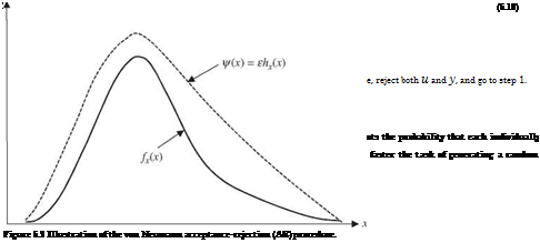
acceptance-rejection (AR) method is to replace the original fx(x) by an appro­priate PDF hx(x) from which random variates can be produced easily and ef­ficiently. The generated random variate from hx(x), then, is subject to testing before it is accepted as one from the original fx (x). This approach for generating random numbers has become widely used.

In AR methods, the PDF fx (x) from which a random variate x to be generated is represented, in terms of hx(x), by

fx (x) = ehx (x)g(x) (6.9)

Acceptance-rejection methods

in which є > 1 and 0 < g(x) < 1. Figure 6.2 illustrates the AR method in that the constant є > 1 is chosen such that f (x) = єhx (x) over the sample space of the random variable X. The problem then is to find a function f (x) = єhx(x) such that f (x) > fx(x) and a function hx(x) = f (x)^, from which random variates are generated. The constant є that satisfies f (x) > fx(x) can be obtained from

(see Problem 6.4). Intuitively, the maximum achievable efficiency for an AR method occurs when f (x) = fx(x). In this case, є = 1, g(x) = 1, and the corre­sponding probability of acceptance P {U < g(Y)} = 1. Therefore, consideration must be given to two aspects when selecting hx(x) for AR methods: (1) the ef­ficiency and exactness of generating a random number from hx(x) and (2) the closeness of hx(x) in imitating fx(x).

Acceptance-rejection methods

Example 6.3 Consider that Manning’s roughness coefficient X of a cast iron pipe is uncertain with a density function fx(x), a < x < b. Develop an AR algorithm using f (x) = c and hx(x) = 1/(b — a), for a < x < b.

1. Generate ui from U(0, 1).

2. Generate U2 from U(0, 1) from which y = a + (b — a)u2.

3. Determine if

Подпись: U1 < g(y) =fx [a + (b — a)u2]

c

holds. If yes, accept y; otherwise, reject (U1, y), and return to step 1.

In fact, this is the von Neumann (1951) algorithm for the AR method.

AR methods are important tools for random number generation because they can be very fast in comparison with the CDF-inverse method for distribution models the analytical forms of CDF inverse of which are not available. This approach has been applied to some distributions, such as gamma, resulting in extremely simple and efficient algorithms (Dagpunar, 1988).

Classifications of Random Variates Generation Algorithms

6.1.1 CDF-inverse method

Let a random variable X have the cumulative distribution function (CDF) Fx(x). From Sec. 2.3.1, Fx(x) is a nondecreasing function with respect to the value of x, and 0 < Fx(x) < 1. Therefore, F-1(u) may be defined for any value of u between 0 and 1 as F-1(u) is the smallest x satisfying Fx(x) > u.

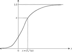
For the majority of continuous probability distributions applied in hydrosys­tems engineering and analysis, Fx(x) is a strictly increasing function of x. Hence a unique relationship exists between Fx (x) and u; that is, u = Fx (x), as shown in Fig. 6.1. Furthermore, it can be shown that if U is a standard uniform ran­dom variable defined over the unit interval [0, 1], denoted by U ~ U(0,1), the following relationship holds:

X = Fx-1(U) (6.6)

Note that X is a random variable because it is a function of the random variable U. From Eq. (6.6), the one-to-one correspondence between X and U, through the CDF, enables the generation of random numbers X ~ Fx(x) from the standard uniform random numbers. The algorithm using the CDF-inverse method for generating continuous random numbers from a CDF Fx(x) can be stated as follows:

1. Generate n uniform random numbers u1, u2,…, un from U(0,1).

2. Solve for xi = F-1(ui), for і = 1, 2,…, n.

Fx(x) = u

Classifications of Random Variates Generation Algorithms

Figure 6.1 Schematic diagram ofthe inverse-CDF method for generating random variates.

Example 6.1 Consider that the Manning roughness coefficient X of a cast iron pipe is uncertain, having a uniform distribution fx(x) = 1/(6 — a), a < x < b. Develop an algorithm using the CDF-inverse method to generate a random Manning roughness coefficient.

Classifications of Random Variates Generation Algorithms
Подпись: A simple algorithm for generating uniform random variates from U(a, b) is 1. Generate n standard uniform random variates ui, u2,..., un from U(0,1). 2. Calculate the corresponding uniform random variates xi = a + (b — a)ui, i = 1, 2,..., n.
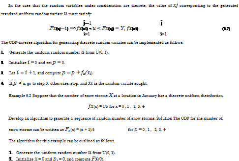
Подпись: In the case that the random variables under consideration are discrete, the value of xj corresponding to the generated standard uniform random variate u must satisfy j—1 j Fx(xj—1) = ^ fx(xi) < u < Fx(xj) = Y, fx(xi) (6.7) i=1 i=1 The CDF-inverse algorithm for generating discrete random variates can be implemented as follows: 1. Generate the uniform random number u from U(0, 1). 2. Initialize i = 0 and set p = 0. 3. Let i = i + 1, and compute p = p + fx(xi). 4. If p < u, go to step 3; otherwise, stop, and xi is the random variate sought. Example 6.2 Suppose that the number of snow storms X at a location in January has a discrete uniform distribution fx(x) = 1/5 for x = 0,1, 2, 3, 4 Develop an algorithm to generate a sequence of random number of snow storms. Solution The CDF for the number of snow storms can be written as Fx(x) = (x + 1)/5 for x = 0,1, 2, 3, 4 The algorithm for this example can be outlined as follows. 1. Generate the uniform random number u from U(0, 1). 2. Initialize x = 0 and p1 = 0, and compute Fx(0).

Solution Using the CDF-inverse method, the expression of the CDF of the random variable is first sought. The CDF for this example can be derived as

3. Test if pi < u < Fx(x). If yes, x is the solution; otherwise, go to step 4.

4. Let p1 = Fx(x), x = x + 1, and compute Fx(x + 1). Go to step 3.

To apply the CDF-inverse method for generating random numbers efficiently, an explicit expression between X and U is essential so that X can be obtained analytically from the generated U. The distributions the inverse forms of which are analytically expressible include exponential, uniform, Weibull, and Gumbel. Table 6.3 lists some distributions that are used in hydrosystems the CDF in­verses of which are analytically expressible.

When the analytical forms of the CDF inverse are not available, applying the CDF-inverse method would require solving

/

x

fx (t) dt (6.8)

-TO

for x from the known u. For many commonly used distributions such as normal, lognormal, and gamma, solving Eq. (6.8) is inefficient and difficult. More effi­cient algorithms have been developed to generate random variates from those distributions; some of these are described in Sec. 6.4.