Control-variate method

The basic idea behind the control-variate method for variance reduction is to take advantage of the available information for the selected variables related to the quantity to be estimated. Referring to Eq. (6.91), the quantity G to be estimated is the expected value of the output of the model g(X). The value of G can be estimated directly by those techniques described in Sec. 6.6. However, a reduction in estimation error can be achieved by indirectly estimating the mean of a surrogate model g(X, Z) as (Ang and Tang, 1984)

g(X, Z) = g(X) — Z(g'(X) — E[g'(X)]} (6.100)

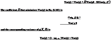
in which g'(X) is a control variable with the known expected value E[g'(X)], and Z is a coefficient to be determined in such a way that the variance of g(X, Z) is minimized. The control variable g'(X) is also a model, which is a function of the same stochastic variables X as in the model g(X). It can be shown that g(X, Z) is an unbiased estimator of the random model output g(X), that is, E[g(X, Z)] = E[g(X)] = G. The variance of g(X, Z), for any given Z, can be obtained as

in which pg, gі is the correlation coefficient between the model output g(X) and the control variable g'(X). Since both model output g(X) and the control vari­able g ‘(X) depend on the same stochastic variables X, correlation to a certain degree exists between g(X) and g'(X). As can be seen from Eq. (6.103), using a control variable g ‘(X) could result in a variance reduction in estimating the expected model output. The degree of variance reduction depends on how large the value of the correlation coefficient is. There exists a tradeoff here. To attain a high variance reduction, a high correlation coefficient is required, which can be achieved by making the control variable g'(X) a good approximation to the model g(X). However, this could result in a complex control variable for which the expected value may not be derived easily. On the other hand, the use of a simple control variable g'(X) that is a poor approximation of g(X) would not result in an effective variance reduction in estimation.

The attainment of variance reduction, however, cannot be achieved from total ignorance. Equation (6.103) indicates that variance reduction for estimating G is possible only through the correlation between g(X) and g'(X). However, the correlation between g(X) and g'(X) is generally not known in real-life situa­tions. Consequently, a sequence of random variates of X must be produced to compute the corresponding values of the model output g(X) and the control variable g'(X) to estimate the optimal value of Z* by Eq. (6.102). The general algorithm of the control-variate method can be stated as follows.

1. Select a control variable g'(X).

2. Generate random variates for X(i) according to their probabilistic laws.

3. Compute the corresponding values of the model g(X(i)) and the control vari­able g’ (X(i)).

4. Repeat steps 2 and 3 n times.

5. Estimate the value Z*, according to Eq. (6.102), by

c En=1(g(° — g)[g/(° — E(gQ]

* n Var(g 0

Z ЕП=1і£(0 — g]fe'(0 — E(g0]

Z* En=1k'(0 — E (g OP

depending on whether the variance of the control variable g ‘(X) is known or not.

6. Estimate the value of G, according to Eq. (6.100), by

G = -]T (g(i) — Z* g/(i)) + Z* e (g о

i=1

Further improvement in accuracy could be made in step 2 of this above algo­rithm by using the antithetic-variate approach to generate random variates.

This idea of the control-variate method can be extended to consider a set of J control variates g'(X) = [g(X), g2(X), …, gJ(X)]г. Then Eq. (6.100) can be modified as

J

g (X, Z) = g (X) -£ Zj {g j (X) — E[g j (X)]} (6.107)

j=1

The vector of optimal coefficients Z*= (Z*nZ*2,… ,Z* J ) that minimizes the vari­ance of g(X, Z) is

in which c is a J x 1 cross-covariance vector between J control variates g'(X) and the model g(X), that is, c = {Cov[g(X),g[(X)],Cov[g(X),g’2(X)], Cov[g(X), g J (X)]}, and C is the covariance matrix of the J control variates, that is, C = [oij] = [ g i (X), g j (X)], for i, j = 1,2,…, J. The corresponding minimum variance of the estimator g(X, Z) is

Var(g) = Var(g) — ctCc= (1 — pgg,) Var(g) (6.109)

in which pg, gі is the multiple correlation coefficient between g(X) and the vector of control variates g'(X). The squared multiple correlation coefficient is called the coefficient of determination and represents the percentage of variation in the model outputs g(X) explained by the J control variates g'(X).