Category Hydrosystems Engineering Reliability Assessment and Risk Analysis

Integration of Reliability in Optimal Hydrosystems Design

8.1 Introduction

All hydrosystems engineering problems involve many interconnected and in­terrelated components. The analysis of any hydrosystem problem should take those interactions into account so that the overall behavior of the system is modeled properly. In general, problems in hydrosystems engineering can be classified into (1) development problems, (2) design problems, and (3) opera­tional problems (Buras, 1972). In fact, practically all hydrosystems engineering problems encompass these problem types, which involve activities relating to determination of (1) the optimal scale of development of the project, (2) the op­timal dimensions of the various components of the system, and (3) the optimal operation of the system.

Frequently, design and analysis of hydrosystems involve the use of models. The primary objectives of modeling exercises are (1) to analyze the behavior of existing systems so as to improve their performance and (2) to identify the “best” structural components and configurations of a system under planning. As discussed in Chap. 1, owing to the existence of various uncertainties in hydrosystems modeling, one cannot be certain that the best solution obtained is indeed truly optimal. The conventional approach when facing uncertainties in engineering design is to conduct sensitivity analysis, by which the influences of variation in model parameters subject to uncertainty on the system responses are assessed quantitatively. Simple sensitivity analyses often are ineffective in providing design, management, or operational guidance because when the various system parameters are changed systematically in sensitivity analysis, no consideration is given to whether the changed values are likely or realistic. It is therefore the objective of this chapter to present some practical approaches that integrate the uncertainties and reliability in an optimization framework for hydrosystems design, management, and operation.

Copyright © 2006 by The McGraw-Hill Companies, Inc. Click here for terms of use.

This chapter starts with a brief description of the concepts of some frequently used optimization techniques in hydrosystems engineering design, manage­ment, and operation. More detailed descriptions of the various optimization techniques are given by Mays and Tung (1992), along with several specialized textbooks on the different subject matters. In Sec. 8.2, focus is placed on some typical problems in the context of resource allocation to optimize system reli­ability. Then the concept of risk-based design is described in Sec. 8.3, followed by an example application to hydrosystems engineering in Sec. 8.4. The last two sections, Secs. 8.5 and 8.6, describe a simple way to solve an optimization model in which the parameters are subject to uncertainty.

Summary and Conclusions

Hwang et al. (1981) presented a review of literature related to system reliability evaluation techniques for small to large complex systems. A large system was defined as one that has more than 10 components and a moderate system as one which has more than 6 components and less than 10. Complex systems were defined as ones that could not be reduced to a series-parallel system. Hwang et al. concluded that for a large, complex system, computer programs should be used that provide the minimum cut sets and calculate the minimal cut approx­imation to system reliability. Minimal paths can be generated from minimum cuts. Based on minimum cut sets, reliability approximations then can be ob­tained for large, complex networks. Hwang et al. also noted that Monte Carlo methods for system reliability evaluation can be used when component relia­bilities are sampled by the Monte Carlo method. They also identified several miscellaneous approaches for evaluating complex systems, including a moment method, a block-diagram method, Bayesian decomposition, and decomposition by Boolean expression.

Hwang et al. (1981) concluded that of all the evaluation techniques in the papers surveyed, only a few had limited success in solving some large, complex

system reliability problems, and few techniques have been completely effective when applied to large system reliability problems. They suggested that a gen­erally efficient graph partitioning technique for reliability evaluation of large, highly interconnected networks should be developed.

Since the 1981 paper by Hwang et al., several other system reliability eval­uation techniques have been reported in the literature. Aggarwal et al. (1982) presented a method that uses decomposition of a probabilistic graph using cut sets. The method is applied to a simplified network with five nodes and seven links, and only limited computational results are presented.

Appendix 7A: Derivation of Bounds for Bivariate Normal Probability

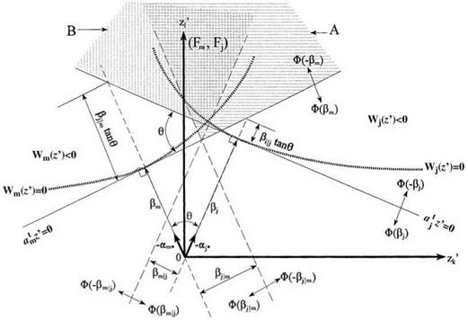
Consider two performance functions Wj (Z’) = 0 and Wm(Z’) = 0 in a two­dimensional standardized, uncorrelated normal space whose design points are z j * and z m*, respectively. At each of the design points, the first-order failure hyperplanes can be expressed as

Wj (Zо = 0 ^ (Z – 4, j*) = aj + ayZ[ + ayZ2 (7A.1)

k=1 ‘ k ‘

2 f d W

Wm(Z0 = 0 ^ ^ 4 rrj, ) (Zk — Zk m*) = a0m + a1mZ1 + a2mZ2 (7A.2)

іґЛd Zkl,

Summary and Conclusions Подпись: Zk,m* Подпись: fork = 1, 2
Summary and Conclusions

in which zk, m* is the coordinate of the kth stochastic basic variable at the design point z’m* of the mth performance function, and

The covariance between the two performance functions can be obtained as

Cov[Wj (Z/), Wm(Z )] = E{[(a0j + a1jZ1 + a2jZ2) — a0j]

x [(a0m + a1mZ1 + a2mZ2) — a0m]}

= E [(a1jZ1 + a2jZ2)(a1mZ1 + a2mZ2)]

= a1ja1m + a2ja2m (7A..3)

Hence the correlation coefficient between the two performance functions at the design points is

Summary and Conclusions

a1ja1m + a2ja2m


(7A.4)


Pjm —


a2j + a!’Va2m + a2m


Подпись: pjm — Summary and Conclusions Подпись: (7A.5)

This can be generalized to multidimensional problems involving M stochastic basic variables as

Подпись: Pjm — Подпись: a1j a2j vj4’ v4-+4 Summary and Conclusions Summary and Conclusions

Note that the preceding correlation coefficient between the two performance functions Pjm is exactly equal to the inner product of the corresponding direc­tional derivative vectors

Подпись: (7A.6) ( aj*) ( am*) — (aj*) (am*)

— |aj||am*| cos в

— cos в

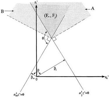
in which в is the angle between the directional derivatives of the two perfor­mance functions. Hence, if the two performance functions are positively cor­related, the angle в between am* and aj * lies in the range 0° < в < 90°. On the other hand, negative correlation between Wj (Z) and Wm(Z) corresponds to the range 90° < в < 180°. Plots for positively and negatively correlated performance functions are show in Figs. 7A.1 and 7A.2, respectively.

When Wj (Z) and Wm(Z) are positively correlated, that is, pjm > 0, referring to Fig. 7A.1, the shaded area representing the joint failure of the two perfor­mance functions satisfies the following relationships:

(Fj, Fm) э A and (Fj, Fm) э B

in which (Fj, Fm) represents the joint failure events of the two performance functions, and sets A and B are defined in Fig. 7A.1.

Again, referring to Fig. 7A.1, the following relationship holds:

Max[P(A), P (B)] < P(Fj, Fm) < P(A) + P (B) (7A.7)

By orthogonality, one has

P (A) — Ф(-Pm)Ф(Pj | m) (7A.8)

P (B) — Ф(вj m, Pmj) (7A.9)

1 n ej — pjmfim „ Pm — pmjPj. л лл

where Pj | m — , =- Pm | j — , = (7A.10)

V 1 — Pjm у 1 — pmj

which are defined in Fig. 7A.1.

Summary and Conclusions

Figure 7A.1 Two intersecting tangent planes with positively correlated failure events. (Ang and Tang, 1984.)


Figure 7A.2 Two intersecting tangent planes with negatively correlated fail­ure events. (Ang and Tang, 1984.)


Summary and Conclusions

Referring to Fig. 7A.2 for negatively correlated Wj (Z) and Wm(Z), it can be observed that

(Fj, Fm) c A and (Fj, Fm) c B

resulting in

0 < P(Fj, Fm) < min[P(A), P(B)] (7A.11)

Подпись: Problems
with P(A) and P(B) given in Eqs.(7A.8) and (7A.9), respectively.

7.1

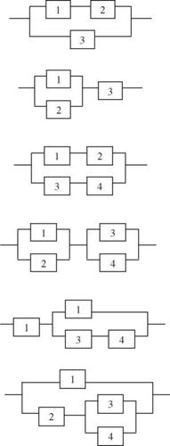
Summary and Conclusions Подпись: Figure 7P.1 Configuration of var-ious systems for Problem 7.1.
Summary and Conclusions

Derive the expression of system reliability for the system configurations shown in Fig. 7P.1 under the condition of (a) all units are dependent and different and (b) all units are independent and identical.

7.2 Consider that two independent, identical units are to be added to an existing unit that would result in three units in the whole system.

(a) Sketch all possible system configurations according to the arrangement of the three units.

(b) Rank your system configurations according to the system reliability.

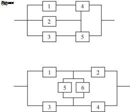
7.3 Consider the two system configurations shown in Fig. 7P.2. Use the cut-set method to determine the system reliability. Assume that all system components are iden­tical and behave independently of each other.

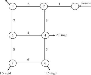
7.4 Consider a hypothetical water distribution network consisting of two loops, as shown in Fig. 7P.3. Let’s say that the service failure of the system is when at least one demand node cannot receive water. (a) Construct a tree diagram indi­cating failure cases for the water distribution network. (b) Determine the system reliability if all pipe sections behave independently, and each has a breakage probability of 0.03.

7.5 Resolve Problem 7.4 by cut-set analysis.

7.6 Resolve Problem 7.4 by tie-set analysis

7.7 Resolve Problem 7.4 by the conditional probability approach.

7.8 Summary and Conclusions
A detention basin is designed to accommodate excessive surface runoff temporar­ily during storm events. The detention basin should not overflow, if possible, to prevent potential pollution of the stream or other receiving water bodies. For simplicity, the amount of daily rainfall is categorized as heavy, moderate, and light (including none). With the present storage capacity, the detention basin is capable of accommodating runoff generated by two consecutive days of heavy rainfall or three consecutive days of at least moderate rainfall. The daily rainfall amounts around the detention basin site are not entirely independent. In other

Summary and Conclusions

2.5 mgd

Figure 7.3 Hypothetical water distribution network.

words, the amount of daily rainfall on a given day would affect the daily rainfall amount on the next day. Let random variable Xt represent the amount of rain­fall on any day t. The transition probability matrix, indicating the conditional probability of rainfall amount in a given day t conditioned on the rainfall amount of the previous day t — 1, is shown in the following table (after Mays and Tung 1992).

Xt+1

Heavy (H)

Moderate (M)

Light (L)

X t Heavy (H)

0.3

0.5

0.2

Moderate (M)

0.3

0.4

0.3

Light (L)

0.1

0.3

0.6

Fault-tree analysis

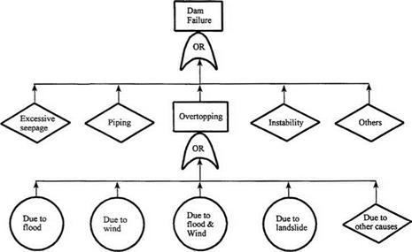
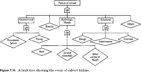
Conceptually, fault-tree analysis, unlike event-tree analysis, is a backward anal­ysis that begins with a system failure and traces backward, searching for pos­sible causes of the failure. Fault-tree analysis was initiated at Bell Telephone Laboratories and Boeing Aircraft Company (Barlow et al., 1975). Since then, it has been used for evaluating the reliability of many different engineering systems. In hydrosystems engineering designs, fault-tree analysis has been ap­plied to evaluate the risk and reliability of earth dams, as shown in Fig. 7.14 (Cheng, 1982), underground water control systems (Bogardi et al., 1987), and water-retaining structures including dikes and sluice gates (Vrijling, 1987, 1993). Figure 7.15 shows a fault tree for the failure of a culvert as another example.

A fault tree is a logical diagram representing the consequence of the compo­nent failures (basic or primary failures) on the system failure (top failure or

Fault-tree analysis

Figure 7.14 Simple fault tree for failure of existing dams. (After Cheng, 1982.)

Fault-tree analysis

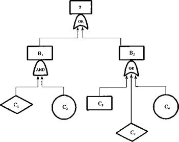
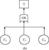
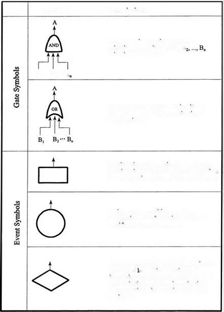
top event). A simple fault tree is given in the Fig. 7.16a as an example. Two major types of combination nodes (or gates) are used in a fault tree. The AND node implies that the output event occurs only if all the input events occur simultaneously, corresponding to the intersection operation in probability the­ory. The OR node indicates that the output event occurs if any one or more of the input events occur, i. e., a union. The two and three other frequently used event notations are shown in Fig. 7.17. Boolean algebra operations are used in fault-tree analysis. Thus, for the fault tree shown in Fig. 7.16,

B1 = C1 П C2 B2 = C3 U C4 U C1

Hence the top event is related to the component events as

T = B1 U B2 = (C1 П C2) U (C3 U C4 U C1) = C1 U C3 U C4

Thus the probability of the top event occurring can be expressed as

P(T) = P(C1U C3 U C4)

If C1, C3, and C4 are mutually exclusive, then

P (T) = P (C1) + P (C3) + P (C4)

Hence Fig. 7.16a can be reduced to an equivalent but simpler fault tree as Fig. 7.16b. System reliability ps, sys(t) is the probability that the top event does not occur over the time interval (0, t].

Dhillon and Singh (1981) pointed out the advantages and disadvantages of the fault-tree analysis technique. Advantages include

1. It provides insight into the system behavior.

2. It requires engineers to understand the system thoroughly and deal specifi­cally with one particular failure at a time.

Fault-tree analysis

(a)

Fault-tree analysis

Figure 7.16 An example fault tree: (a) original fault tree before simplifi­cation; (b) reduced fault tree.

3. It helps to ferret out failures deductively.

4. It provides a visible and instructive tool to designers, users, and management to justify design changes and tradeoff studies.

5. It provides options to perform quantitative or qualitative reliability analysis.

6. The technique can handle complex systems.

7. Commercial codes are available to perform the analysis.

Disadvantages include

1. It can be costly and time-consuming.

2. Results can be difficult to check.

Fault-tree analysis

Descriptions


Symbol


Fault-tree analysis

B, B2-B


Fault-tree analysis
Fault-tree analysis
Fault-tree analysis
Fault-tree analysis

Figure 7.17 Some basic node symbols used in fault-tree analysis.


Fault-tree analysis

Fault-tree analysis

3. The technique normally considers that the system components are in either working or failed state; therefore, the partial failure stats of components are difficult to handle.

4. Analytical solutions for fault trees containing standbys and repairable com­ponents are difficult to obtain for the general case.

5. To include all types of common failure causes requires considerable effort.

Fault-tree construction. Before constructing a fault tree, engineers must thor­oughly understand the system and its intended use. One must determine the higher-order functional events and continue the fault event analysis to deter­mine their logical relationships with lower level events. Once this is accom­plished, the fault-tree can be constructed. A brief description of fault-tree construction is given in the following paragraphs. The basic concepts of fault – ree analysis are presented in Henley and Kumamoto (1981) and Dhillon and Singh (1981).

The major objective of fault-tree construction is to represent the system con­dition that may cause system failure in a symbolic manner. In other words, the fault tree consists of sequences of events that lead to system failure. There are actually two types of building blocks: gate symbols and event symbols.

Gate symbols connect events according to their causal relation such that they may have one or more input events but only one output event. Figure 7.17 shows the two commonly used gate symbols and three types of commonly used event symbols. A fault event, denoted by a rectangular box, results from a combina­tion of more basic faults acting through logic gates. A circle denotes a basic component failure that represents the limit of resolution of a fault tree. A dia­mond represents a fault event whose causes have not been fully developed. For more complete descriptions on other types of gate and event symbols, readers are referred to Henley and Kumamoto (1981).

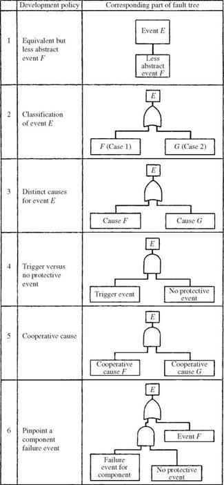
Henley and Kumamoto (1981) presented heuristic guidelines for constructing fault trees, and these are summarized in Table 7.1 and Fig. 7.18 and are listed below:

1. Replace abstract events by less abstract events.

2. Classify an event into more elementary events.

3. Identify distinct causes for an event.

4. Couple trigger events with “no-protection actions.”

5. Find cooperative causes for an event.

6. Pinpoint component failure events.

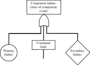
7. Develop component failure using Fig. 7.18.

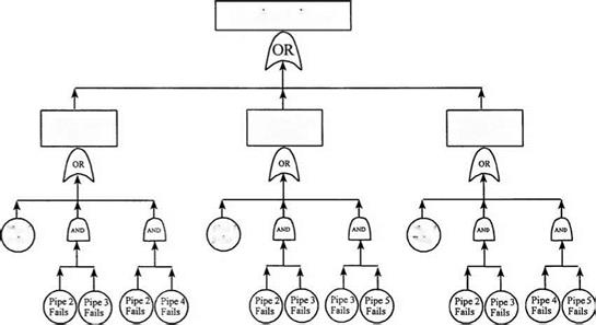
Figure 7.19 shows a fault tree for the example pipe network of Fig. 7.9.

Fault-tree analysis

Source: Henley and Kumomoto (1981).

Fault-tree analysis

Figure 7.18 Development of component failure. (Henley and Kumomoto, 1981.)


Fault-tree analysis

Evaluation of fault trees. The basic steps used to evaluate fault trees include

(1) construction of the fault tree, (2) determination of the minimal cut sets, (3) development of primary event information, (4) development of cut-set infor­mation, and (5) development of top event information.

Fault-tree analysis Подпись: User з Not Serviced Fault-tree analysis Fault-tree analysis Подпись: User 5 Not Serviced

To evaluate the fault tree, one always should start from the minimal cut sets that in essence, are critical paths. Basically, the fault-tree evaluation consists of two distinct processes: (1) determination of the logical combination of events

Figure 7.19 Fault tree for reliability analysis of example pipe network in Fig. 7.9.

that cause top event failure expressed in the minimal cut sets and (2) numerical evaluation of the expression.

Cut sets, as discussed previously, are collections of basic events such that if all these basic events occur, then the top event is guaranteed to occur. The tie set is a dual concept to the cut set in that it is a collection of basic events of which if none of the events in the tie set occur, then the top event is guaranteed not to occur. As one could imagine, a large system has an enormous number of failure modes. A minimal cut set is one that if any basic event is removed from the set, the remaining events collectively are no longer a cut set. By the use of minimum cut sets, the number of cut sets and basic events are reduced in order to simplify the analysis.

The system availability Asys(t) is the probability that the top event does not occur at time t, which is the probability of the systems operating successfully when the top event is an OR combination of all system hazards. System unavail­ability Usys(t), on the other hand, is the probability that the top event occurs at time t, which is either the probability of system failure or the probability of a particular system hazard at time t.

System reliability ps, sys(t) is the probability that the top event does not occur over time interval (0, t). System reliability requires continuation of the nonoc­currence of the top event, and its value is less than or equal to the availability. On other hand, the system unreliability, pf, sys(t) is the probability that the top event occurs before time t and is complementary to the system reliability. Also, system unreliability, in general, is greater than or equal to system unavail­ability. From the system unreliability, the system failure density f sys(t) can be obtained according to Eq. (5.2).

Conditional probability approach

This approach starts with a selection of key components and modes of opera­tion whose states (operational or failure) would decompose the entire system into simple series and/or parallel subsystems for which the reliability or failure probability can be evaluated easily. Then the reliability of the entire system is obtained by combining those of the subsystems using the conditional probability rule as

ps, sys — ps | Fm x ps, m + ps | Fm x pf, m (T.65)

in which ps | and ps | Fm are the conditional system reliabilities given that the

mth component is operational Fm and failed Fm, respectively, and ps, m and pf, m are the reliability and failure probabilities of the mth component, respectively.

Except for very simple and small systems, a nested conditional probability operation is inevitable. Efficient evaluation of system reliability of a complex system hinges entirely on a proper selection of key components, which generally is a difficult task when the scale of the system is large. Furthermore, the method cannot be adapted easily to computerization for problem solving.

Example 7.15 Find the system reliability of the water distribution network in Fig. 7.9 using the conditional probability approach.

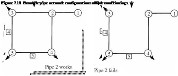
Solution Using the conditional probability approach for system reliability evaluation, first select pipe section 1 as the key element that decomposes the system into a simpler
configuration, as shown in Fig. 7.13. After the entire system is decomposed into a simple system configuration, the conditional probability of the decomposed systems can be evaluated easily. For example, the conditional system reliability, after imposing F1 and F3 for pipes 1 and 3, respectively, can be expressed as

Ps, sys | F[,F3 = P(F2 n F4n F5) = (0.95)3 = 0.8574

where ps | f ‘,f3 is conditional system reliability. Conditional system reliabilities for other imposed conditions are shown in Fig. 7.13. After the conditional system re­liabilities for the decomposed systems are calculated, the reliability of the entire

Conditional probability approach

Original system

system can be combined using Eq. (7.65). For this particular example, the system reliability is

Ps, sys = Ps | F, F3 x P(F1, F3) + Ps | F, F3,F2 x P(F1, F3, F2)

+ Ps | F1,F,,F2 x P (F1> F3, F2)

= (0.8574)(0.95)(0.05) + (0.9975)(0.95)3 + (0.9025)(0.95)2(0.05)

= 0.9367

Path enumeration method

This is a very powerful method for system reliability evaluation. A path is defined as a set of components or modes of operation that leads to a certain outcome of the system. In system reliability analysis, the system outcomes of interest are those of failed state or operational state. A minimum path is one in which no component is traversed more than once in going along the path. Under this methodologic category, tie-set analysis and cut-set analysis are two well-known techniques.

Cut-set analysis. The cut set is defined as a set of system components or modes of operation that, when failed, cause the failure of the system. Cut-set analysis is powerful for evaluating system reliability for two reasons: (1) It can be pro­grammed easily on digital computers for fast and efficient solutions of any general system configuration, especially in the form of a network, and (2) the cut sets are directly related to the modes of system failure and therefore iden­tify the distinct and discrete ways in which a system may fail. For example, in a water distribution system, a cut set will be the set of system components including pipe sections, pumps, storage facilities, etc. that, when failed jointly, would disrupt the service to certain users.

Подпись: pf ,sys — P ( U Cm 1 — P m=1 Подпись: I U m=1 Path enumeration method Подпись: (7.63)

The cut-set method uses the minimum cut sets for calculating the system failure probability. The minimum cut set is a set of system components that, when all failed, causes failure of the system but when any one component of the set does not fail does not cause system failure. A minimum cut set implies that all components of the cut set must be in the failure state to cause system failure. Therefore, the components or modes of operation involved in the minimum cut set are effectively connected in parallel, and each minimum cut set is connected in series. Consequently, the failure probability of a system can be expressed as

in which Cm is the mth of the total I minimum cut sets, Jm is the total number of components or modes of operation in the mth minimum cut set, and Fmj represents the failure event associated with the j th components or mode of operation in the mth minimum cut set. In the case that the number of minimum

cut sets I is large, computing the bounds for probability of a union described in Sec. 7.2.3 can be applied. The bounds on the failure probability of the system should be examined for their closeness to ensure that adequate accuracy is obtained.

Example 7.13 Refer to the simple water distribution network shown in Fig. 7.9 in Example 7.12. Evaluate the system reliability using the minimum cut-set method.

Solution Based on the system reliability as defined, the minimum cut sets for the example pipe network are

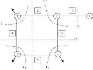
C1 : F1 C2 : F2 П F3 C3 : F2 П F4 C4 : F3 П F5

C5 : F4 П F5 C6 : F2 П F5 C7 : F3 П F4

where Cm is the mth cut set, and Fk is the failure state of pipe link k. The seven cut sets for the example network listed above are shown in Fig. 7.11. The system unreliability pf, sys is the probability of occurrence of the union of the cut set, that is,

Pf, sys = P U Cm

m=1

The system reliability can be obtained by subtracting pf, sys from 1. However, the computation, in general, will be very cumbersome for finding the probability of the

C6

Path enumeration method


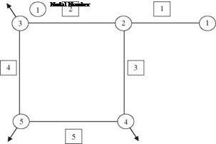
Nodal number


Pipe number


Path enumeration methodPath enumeration method

Cm = The mth cut set

union of large numbers of events, even if they are independent. In this circumstance, it is computationally easier to compute the system reliability as

Ps, sys = 1 — P ( U Cmj = P ( n Cm m=1 J m=1

Since all the cut sets behave independently, all their complements also behave in­dependently. The probability of the intersection of a number of independent events, according to Eq. (2.5), is

Подпись: m=1ps, sys = p( n C’r^j = ^ P(C’m) m=1 /

Подпись: whereP (C1) = 0.95 P (C2) = P (C3) = ••• = P (C’7) = 0.9975

Hence the system reliability of the example water distribution network is ps, sys = (0.95)(0.9975)6 = 0.9360

Path enumeration method Path enumeration method Подпись: mj Подпись: (7.64)

Tie-set analysis. As the complement of a cut set, a tie set is a minimal path of the system in which system components or modes of operation are arranged in series. Consequently, a tie set fails if any of its components or modes of operation fail. All tie sets are effectively connected in parallel; that is, the system will be in the operating state if any of its tie sets are functioning. Therefore, the system reliability can be expressed as

in which T m is the mth tie set of all I tie sets, Jm is the total number of compo­nents or modes of operation in the mth tie set, and F’mj represents the nonfailure state of the j th component in the mth tie set. Again, when the number of tie sets is large, computation of exact system reliability by Eq. (7.64) could be cum­bersome. In such a condition, bounds for system reliability could be computed.

The main disadvantage of the tie-set method is that failure modes are not directly identified. Direct identification of failure modes is sometimes essential if a limited amount of a resource is available to focus on a few dominant failure modes.

Example 7.14 Refer to the simple water distribution network as shown in Fig. 7.9. Use tie-set analysis to evaluate the system reliability.

Solution The minimum tie sets (or path), based on the definition of system reliability given previously, for the example network are

T1 : F1 n F2 n F’4 n F5 T 2 : F1 n F3 n F4 n F5 T 3 : F1 n F2 n F3 n F4 T 4 : F1 n F2 n F3 n F5

where T m is the mth minimum tie set, and F j is the nonfailure of the j th pipe link in the network. The four minimum tie sets are shown in Fig. 7.12. The system reliability, based on Eq. (7.64), is

Ps, sys — P(T 1 U T2 U T3 U T4)

= [P(T1) + P(T2) + P(T3) + P(T4)] – [P(T1, T2) + P(T1, T3)

+ P(T1, T4) + P(T2, T3) + P(T2, T4) + P(T3, T4)]

+ [P(T1, T2, T3) + P(T1, T2, T4) + P(T1, T3, T4) + P(T2, T3, T4)] – P(T1, T2, T3, T4)

Since all pipes in the network behave independently, all minimum tie sets behave independently. In such circumstances, the probability of the joint occurrence of multi­ple independent events is simply equal to the multiplication of the probability of the individual events. That is,

P (T1) — P (F1) P (F2) P (F4) P (F,5) — (0.95)4 — 0.81451

Подпись: —©

Path enumeration method Подпись: <D

Ъ————© ъ

и

Подпись: Яи

T4 = F1 п F 2 n F 3 п F 5

lm = The mth tie set

FJ = Nonfailure state of pipe section j

Similarly,

P (T 2) = P (T 3) = P (T 4) = 0.81451

Note that in this example the unions of more than two minimum tie sets are the intersections of the nonfailure state of all five pipe sections. For example, T1 U T 2 =

(F1 П F2 n F4 П F5) U (F1 n F3 П F4 П F5) = (F1 n F2 n F3 n F4 П F5). The system reliability can be reduced to

Pssys = [P(T1) + P(T2) + P(T3) + P(T4)] – 3P(F1 n F2 n F3 n F4)

= 4(0.81451) – 3(0.95)5 = 0.9367

In summary, the path enumeration method involves the following steps (Henley and Gandhi, 1975):

1. Find all minimum paths. In general, this has to be done with the aid of a com­puter when the number of components is large and the system configuration is complex.

2. Find all required unions of the paths.

3. Give each path union a reliability expression in terms of module reliability.

4. Compute the system reliability in terms of module reliabilities.

Methods for Computing Reliability of Complex Systems

Evaluation of the reliability of simple systems, as described in the preceding section, is generally straightforward. However, many practical hydrosystems engineering infrastructures, such as water distribution systems, have neither series nor parallel configuration. Evaluation of the reliability for such com­plex systems generally is difficult. For some systems, with their components arranged in a complex configuration, it is possible to combine components into groups in such a manner that it appears as in series or in parallel. For other systems, special techniques have to be developed that require a certain degree of insight and ingenuity from engineers. A great deal of work has been done on developing techniques for evaluating the reliability of complex systems. This section describes some of the potentially useful techniques for hydrosystems reliability evaluation.

7.4.1 State enumeration method

The state enumeration method lists all possible mutually exclusive states of the system components that define the state of the entire system. In general,
for a system containing M components, each of which can be classified into K operating states, there will be KM possible states for the entire system. For example, if the state of each of the M components is classified into failed and operating states, the system has 2M possible states.

Once all the possible system states are enumerated, the states that result in successful system operation are identified, and the probability of the occurrence of each successful state is computed. The last step is to sum all the successful state probabilities, which yields the system reliability. This method becomes less and less computationally attractive, as one can imagine, when the number of system components and/or the number of states for each component gets larger.

The tree diagram, such as that in Fig. 7.8, is called an event tree, and the analysis involving the construction of an event tree is referred to as event – tree analysis. As can be seen, an event tree simulates not only the topology of

Yes

Yes

Yes

Yes

Yes

Yes

Land flooded

Yes

Yes

Yes

Yes

Methods for Computing Reliability of Complex Systems

Sabotage Excess


Event


Methods for Computing Reliability of Complex Systems

Rood


(human, leakage


overtops


Methods for Computing Reliability of Complex Systems

Подпись: leveeanimal)

Figure 7.8 An example event tree for land flooding relating to levee performance.

a system but, more important, the sequential or chronologic operation of the system.

Example 7.12 Consider a simple water distribution network consisting of five pipes and one loop, as shown in Fig. 7.9. Node 1 is the source node, and nodes 3, 4, and 5 are demand nodes. The components of this network subject to possible failure are the five pipe sections. Within a given time period, each pipe section has an identical failure probability of 5 percent due to breakage or other causes that require it to be removed from service. The system reliability is defined as the probability that water can reach all three demand nodes from the source. Furthermore, it is assumed that the states of serviceability of each pipe are independent.

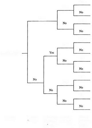
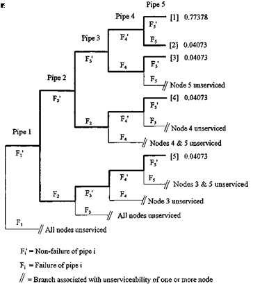
Solution Using the state enumeration method for system reliability evaluation, the associated event tree can be constructed to depict all possible combinations of com­ponent states in the system, as shown in Fig. 7.10. Since each pipe has two possible states, that is, failure F or nonfailure F’, the tree, if fully expanded, would have 25 = 32 branches. However, knowing the role that each pipe component plays in the network connectivity, exhaustive enumeration of all possible states is not necessary.

For example, referring to Fig. 7.10, one realizes that when pipe 1 fails, all demand nodes cannot receive water, indicating a system failure, regardless of the state of the remaining pipe sections. Therefore, branches in the event tree beyond this point do not have to be constructed. Applying some judgment in event-tree construction in this fashion generally can lead to a smaller tree. However, for a complex system, this may not be a trivial task.

Methods for Computing Reliability of Complex Systems

The system reliability can be obtained by summing up the probabilities associ­ated with all of the nonfailure branches. In this example, there are five branches, as

1 Pipe Number

indicated by the heavy lines in the tree, for which all users can have the water deliv­ered by the system. Therefore, the system reliability is

Подпись: = УУ P ( B[m])Подпись:Methods for Computing Reliability of Complex Systems
5

ps, sys = P ( и B[m] m=1

where P (B[m]) is the probability that the branch B[m] of the event tree provides full service to all users. The probability associated with each branch resulting in satisfactory delivery of water to all users can be calculated as the following:

P (B[1]) = P (F1) P (F2) P (F3) P (F4) P (F5)

= (0.95)(0.95)(0.95)(0.95)(0.95) = 0.77378 P (B[2]) = P (F1) P (F2) P (F3) P (F4) P (F5)

= (0.95)(0.95)(0.95)(0.95)(0.05) = 0.04073 P (B[3]) = P (F1) P (F2) P (F3) P (F4) P (F,5)

= (0.95X0.95X0.95X0.05X0.95) = 0.04073

P (B[4]) = P (F[) P (F2) P (F3) P (F4) P (F5)

= (0.95)(0.95)(0.05)(0.95)(0.95) = 0.04073 P (B[5]) = P (F1) P (F2) P (F<3) P (F4) P (F5)

= (0.95)(0.05)(0.95)(0.95)(0.95) = 0.04073

Therefore, the system reliability is the sum of the preceding five probabilities associ­ated with the operating state of the system, which is

ps, sys = 0.77378 + 4(0.04073) = 0.93668

Standby redundant systems

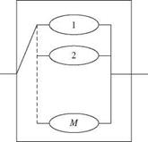
Подпись: Figure 7.7 Standby redundant systems.
Standby redundant systems

A standby redundant system is a parallel system in which only one compo­nent or subsystem is in operation (Fig. 7.7). It is a special case of K-out-of-M system with K = 1. If the operating component fails, then another component is operated. This type of system is different than the parallel system described in Sec. 7.3.2, where all components are concurrently operating because standby

Standby redundant systems Подпись: (7.61)

units do not operate. The system reliability for a system with M components out of which M — 1 units are on standby is the probability that at most M — 1 components fail. This probability can be expressed by

Подпись: MTTF = Подпись: 0 Подпись: Ps,sys(t) dt Подпись: 0 Standby redundant systems Подпись: (7.62)

Note that this equation is valid under the following assumptions: The switching arrangement is perfect, the units are identical, the component failure rates are constant, the standby units are as good as new, and the unit failures are sta­tistically independent. The mean time to failure of the system can be obtained, according to Eq. (5.18), as

Equation (7.62) is intuitively obvious in that the system’s operation is the result of a relay of a series of components. As one component fails, the second one comes to operation until failure occurs. Therefore, the system MTTF is the sum of the MTTFs of individual components.

Example 7.11 As an example of a standby redundant system, assume an exponential failure distribution for two identical pumps, one operating and the second on standby, with identical failure rates of X = 0.0005 failures/h. The standby unit is as good as new at time t = 0. The system reliability for t = 1000 h is

ps, sys(t = 1000) = [1 + (0.0005)(1000)]e—(00005)(1000) = 0.9098

K-out-of-ДО parallel systems

This is a parallel system of M component for which the system would function if K (K < M) or more components function. This type of system also is called a partially redundant system. The general reliability formula for this system is rather cumbersome. For components having an identical reliability function, that is, ps, m(t) = ps(t), the system reliability and unreliability, when component performances are independent, are

M

Ps, sys(t) = 53 Cm, j [Ps(t)]j [1 – Ps(t)]M-j (7.58a)

j =k

K-1

and pf, sys(t) = ]T Cm, j [Ps(t)]j [1 – Ps(t)]M-j (7.58b)

j =0

in which CM, j = M!/[j!(M – j)!] is a binomial constant. Computationally, whether to calculate ps, sys(t) or pf, sys(t) is dictated by the number of terms
involved in the summation. Furthermore, if the failure density function is an exponential distribution, the system reliability can be expressed as

M

ps, Sys(t) = £ Cm, j (e-Xt)j (1 – e-u)M-j (7.59)

j =k

Подпись: fsys(t) Подпись: d [ps,sys(t)] dt M Y^CM,j [Ps(t)]j [1 j =K Подпись: Ps (t)]M- j Подпись: j Ps(t) Подпись: M - j 1 - Ps(t) Подпись: ft (t) Подпись: (7.60)

The failure density function for the system f sys(t) based on the system reli­ability in Eq. (7.58a) is

The availability and unavailability of the system can be obtained from sub­stituting component availability for component reliability in Eqs. (7.58a) and (7.58b), respectively.

Example 7.10 As an example of a K-out-of-M system, consider a pumping system with three pumps, one of which is on standby, all with constant failure rates of X = 0.0005 failures/h. The system reliability for t = 1000 h, M = 3, and K = 2 is

ps, sys(t = 1000) = c3,2(e-(a0005>(1000>)2(1 – е-(0-0005)(шю)) + Сз, з(е-(0’0005)(1000))3

= 3(e-(0.0005)(1000))2 _ 2(e-(0.0005)(1000))3

= 1.1036 – 0.4463 = 0.6573

Parallel systems

For a parallel system, the entire system would perform satisfactorily if any one or more of its components or modes of operation is functioning satisfactorily; the entire system would fail only if all its components or modes of operation fail.

In the framework of load-resistance interference for different modes of oper­ation, the failure probability of a parallel system, according to Eq. (7.9), is

Parallel systems

M

П (Wm < 0)

m=1


Pf, sys = P


P


П (Zm < m=1


вт)


Ф(-в I Rz)


(7.43)


Parallel systems

which can be computed as the multivariate normal probability discussed in Sec. 2.7.2. The bounds for system failure probability also can be computed if the exact value of Pf, sys is not required. In the case that all performance variables W’s are independent, the system failure probability reduces to

M

Pf, sys = П ®(-Pm) (7.44)

m=1

Подпись: ps,sys — P Подпись: M U (Wm m—1 Подпись: > 0) Подпись: P Подпись: M U (Zm > -Pm) m—1 Подпись: (7.45)

Alternatively, the reliability of a parallel system can be expressed as

Подпись: ps,sys Parallel systems Подпись: (7.46)

The second-order bounds for this system reliability, according to Eq. (7.27), are

in which L( jij, em 1 pjm) — P [Zj > ej, Zm > em — Ф( ej, em 1 pjm) +

Ф(в j) + Ф^)-!.

Example 7.8 Referring to Example 7.6, determine the system reliability by consid­ering that the system would fail if all three modes of operation fail.

Solution Since the system is in parallel, the system failure probability can be calculated as

Pf, sys — P(Wi < 0, W2 < 0, W3 < 0)

— P(Z1 < -2.68, Z2 < -3.46, Z3 < -2.68) — 0.0001556

which is obtained in Example 7.6. Hence the reliability of the system is 0.9998444.

In the framework of time-to-failure analysis, the unreliability of a parallel system involving M independent components can be computed as

M

Подпись:pf, sys(t) — ^ pf, m(t)

m—1

in which pf, m(t) — P(Tm < t), the unreliability of the mth component within the specified time interval (0, t]. Hence the system reliability in time interval (0, t] is

M

Ps, sys(t) = 1 – Pf, sys(t) = 1 – П Pf, m(t) (7.48)

m=l

Подпись: and Parallel systems Parallel systems

The failure density function f sys(t) and failure rate hsys(t) for a parallel system consisting of M independent components are

For each component having an exponential failure density function with the parameter Xm, for m — 1,2,…, M, the failure probability of a parallel system can be computed as

M

Pf ,sys(t) — П (1 – e~lmt) (7.51)

m—1

with the corresponding system reliability

M

Ps, sys(t) — 1 – П (1 – e-lmt) (7.52)

m—1

Подпись: M f sys(t) — m—1 Подпись: M Ц(1 - e-jt) j —m Подпись: Xm e Подпись: Xm* Подпись: (7.53)

The system failure density function f sys(t) is

Parallel systems Подпись: (7.54)

In the case that all components have an identical failure rate, that is, X1 — X2 — ■ ■ — XM — X, the MTTF of the system is

The unavailability of a parallel system involving M independent compo­nents is

M

Usys(t) —Ц Um(t) (7.55a)

m—1

and the corresponding system availability is

M

Asys(t) = 1 – Ц Um(t) (7.55b)

m=1

Parallel systems Подпись: (1 - e Подпись: ) Подпись: (7.56)

Under the condition of independent exponential repair functions for the M components, the unavailability of a parallel system is

Parallel systems Parallel systems Подпись: MTTRm MTTRm + MTTFm Подпись: (7.57)

and the stationary system unavailability is

Example 7.9 As an example of a parallel system, consider a pumping station con­sisting of two identical pumps operating in a redundant configuration so that either pump could fail, and the peak discharge could still be delivered. Both pumps have a failure rate of k = 0.0005 failures/h, and both pumps start operating at t = 0. The system reliability for a mission time of t = 1000 h, according to Eq. (7.52), is

Подпись:

Подпись: 15 = 1.5 k
Подпись: = 3000 h

ps, sys(t = 1000) = 1 – (1 – e-(0 0005>(1000>)(1 – e-(0-0005)(1000)) = 0.8452 The MTTF, according to Eq. (7.53), is

Reliability of Simple Systems

In this section the reliability of some simple systems will be discussed. In the framework of time-to-failure analysis, availability of such systems will be pre­sented. Information such as this is essential to serve as the building blocks for determination of reliability or availability of more complex systems.

7.3.1 Series systems

A series system requires that all its components or modes of operation perform satisfactorily to ensure a satisfactory operation of the entire system. In the context of load-resistance interference, the failure event associated with a mode of operation is

Fm = {Wm < 0} form = 1, 2,…, M

in which Wm is the random performance variable associated with the mth mode of operation. Referring to Chap. 4, the failure probability and reliability asso­ciated with the mth mode of operation, respectively, are

P (Fm) = P ( Wm < 0) = P (Zm < ~Pm) = ®(-fim) (7.28a)

P (Fm) = P ( Wm > 0) = P (Zm > – Pm) = 4Pm) (7.28b)

in which Zm is the standard normal random variable associated with Wm, and pm is the reliability index associated with the mth mode of operation.

The failure probability of a series system involving M modes of operation, according to Eq. (7.1), can be expressed as

M

U (Wm < 0)

m=1


Pf, sys = P


P


U (Zm <

m=1


вт)


(7.29)


Reliability of Simple Systems

Reliability of Simple Systems Подпись: (7.30)

Because all the standardized normal random variables Zm’s generally are cor­related, computation of the exact system failure probability using Eq. (7.29) may not be practical, especially when the number of modes of operation M is large. For this case, the second-order bounds for Pf, sys could be viable. According to Eq. (7.26), the bounds for system failure probability are

in which Ф(—вj, —em I Pjm) is the bivariate normal probability, which can be computed by procedures described in Sec. 2.7.2, with Pjm being the correlation coefficient between the performance variables Wj and Wm for the j th and mth modes of operation. Accordingly, the bounds on reliability of a series system can be obtained easily by using Eq. (7.11b).

Подпись: Ф( в j , em 1 pjm > 0) Подпись: <Ф( —emW—ЄІ | m) + Ф(—вj )Ф( — вm | j ) > max[Ф( — вm)Ф(—вj I m), Ф(—вj )Ф( — вm | j )] Подпись: (7.31)

Although computation of the exact bivariate normal probability can be ob­tained through numerical integration, sometimes information about its bounds is sufficient. Under a positively correlated case, narrow bounds of Ф(—вj, —em I Pjm > 0) that require evaluations of only univariate normal probabilities are

where ві Im = в, Ртв" (7.32a)

v/irpm

emu = em,— P’"’m’ (7.32b)

j

In the case that the pair of performance functions is negatively correlated, the bounds for joint failure probability are

0 < Ф(— Єі, —em I Pjm < 0) < minm—emm—ej | m), Ф( — в} m—em | j )] (7.33)

The derivations of Eqs.(7.31) and (7.33) are given in Appendix 7A. Ang and Tang (1984) pointed out that use of an approximation of Eq. (7.31) could improve (tighten) the second-order bound of Eq. (7.30) when the single-mode failure probabilities are small, say, on the order of 10—4. However, if the single-mode
failure probabilities are all large (e. g., 10-2), the bound of Eq. (7.31) will be wide.

Reliability of Simple Systems Подпись: M n m=1 Подпись: P Подпись: П (Zm > Pm) m=1 Подпись: (7.34)

In fact, the reliability of a series system can be computed, according to Eq. (7.2), as

It should be pointed out that, in general, P [n(Zm > —em)] = P [n(Zm < fim)] unless for the univariate case. As can be seen, the reliability of a series system is the multivariate normal probability whose determination can be made by Ditlevsen’s approach, described in Sec. 2.7.2, or by various bounding approaches discussed in Sec. 2.7.3.

Example 7.6 Consider a system consisting of three modes of operation, each of which is specified by the following linear performance functions:

W1( X) = X1 + 2 X2

W2( X) = X1 + X2 + X3

W3( X) = X2 + 2X3

in which the stochastic basic variables X1, X2, and X3 are multivariate normal ran­dom variables with the vector of means

Vx = (М1, М2, М3/ = (6, 6, 6/

and covariance matrix

■9.00

0.00

0.00

Cx =

0.00

9.00

0.00

.0.00

0.00

9.00

The state of the system is such that if any of the three modes of operation fail, the system would fail. Calculate the system reliability.

Solution From the preceding covariance matrix Cx, it is understood that all three stochastic basic variables are uncorrelated, each with a variance of 9, that is, Var(X1) = Var(X2) = Var(X3) = 9. The vector of expected values of W1, W2, and W3 is

Vw = (Mw1, Mw2, Mw3) = [6 + 2(6), 6 + 6 + 6, 6 + 2(6)/ = (18, 18, 18/

The covariance matrix of the three performance functions W’s can be computed as

Cw = S1 Cx S

in which S, the sensitivity matrix, is an K x M matrix, with M and K being the number of performance functions and stochastic basic variables, respectively. The sensitivity matrix S contains, in each column, the vector of sensitivity coefficients for each performance function with respect to individual stochastic basic variable, that is,

S = [S1, 82,…, sm ]

for m = 1,2,…, M. In this example, since all performance functions are linear, the sensitivity matrix consists of coefficients in the performance functions, that is,

1

2

0

s1 =

1

1

1

1

0

1

to 1

Hence the covariance matrix of the three performance functions can be obtained as

45

27

18

Cw =

27

27

27

18

27

45

As can be seen, even though the three stochastic basic variables are uncorrelated, the three performance functions are correlated because they are defined by some stochastic basic variables common to the other performance functions. Hence the variances of W1, W2, and W3 appear on the diagonal of Cw, namely,

Var( W1) = 45 Var( W2) = 27 and Var( W3) = 47

The corresponding correlation matrix of random W’s can be obtained easily as

‘1.000 0.7746 0.4000’

Подпись: RПодпись: w

Подпись: with Подпись: dWm dWm dWm dX 1, dX2’, d XK
Подпись: s

0.7746 1.000 0.7746

0.4000 0.7746 1.000

The system failure probability is defined as

pf ,sys = P [(W1 < 0) U (W2 < 0) U (W3 < 0)]

= P [(Z1 < -2.68) U (Z2 < -3.46) U (Z3 < -2.68)]

The exact system failure probability can be obtained as pf sys = P [(Z1 < -2.68) U (Z2 < -3.46) U (Z3 < -2.68)]

= [P(Z1 < -2.68) + P(Z2 < -3.46) + P(Z3 < -2.68)]

– [P(Z1 < -2.68, Z2 < -3.46) + P(Z1 < -2.68, Z3 < -2.68)

+ P(Z2 < -3.46, Z3 < -2.68)] + P(Z1 < -2.68, Z2 < -3.46, Z3 < -2.68)

= (0.003681 + 0.0002701 + 0.003681) – (0.0001659 + 0.0001987 + 0.0001659) + 0.0001556 = 0.0072572

Hence the system reliability ps>sys = 1 – 0.0072572 = 0.9927428. Note that the preceding bivariate normal probabilities are calculated by Eq. (2.121), whereas the trivariate normal probability is computed according to Ditlevsen’s algorithm using Taylor expansion described in Sec. 2.7.2.

Alternatively, the second-order bounds for the system failure probability can be computed according to Eq. (7.30). The results are

0.007102 < pf, sys < 0.007268

and the corresponding bounds on the system reliability ps, sys are

0.992732 < ps, sys < 0.992898

In the framework of time-to-failure analysis, the reliability ps, m(t) and failure probability pf, m(t) of the mth component over the time interval (0, t ], according to Eqs. (5.1a) and (5.1b), are

/

TO

fm(r) dr (7.35a)

and P(Fm) = pf, m(t) — [ fт(т)dx (7.35b)

70

respectively, where f m(t) is the failure density function for the mth component.

Подпись: ps,sys(t) — P Подпись: M n Fm m=1 Reliability of Simple Systems Подпись: (7.36)

In the case that the performance of individual components is independent of each other, the reliability of a series system is

Similarly, the availability of a series system involving M independent compo­nents is

M

Asys(t) — Ц Am(t) (7.37)

m—1

in which Aeys(t) and Am(t) are availabilities of the entire system and the mth component, respectively, at time t.

Подпись: and Reliability of Simple Systems Reliability of Simple Systems Подпись: fm(t) Подпись: (7.38) (7.39)

According to Eqs. (5.2) and (5.3), the failure density function f sys(t) and the failure rate hsys(t) for a series system involving M independent components can be derived, respectively, as

For the special case of an exponential failure density function such as

Подпись: f m(t) — Xme lmtfor t > 0, Xm > 0, m — 1,2,…, M

Reliability of Simple Systems Подпись: (7.40a) (7.40b)

the reliability and unreliability of a series system with M independent compo­nents, respectively, are

Reliability of Simple Systems Reliability of Simple Systems Подпись: (7.41a)

Assuming an exponential repair function for each independent component, the availability and unavailability for a series system, according to Eqs. (7.37) and (5.59), are

Подпись: (7.41b)and Usys(t) — 1 Asys(t)

Reliability of Simple Systems Reliability of Simple Systems Reliability of Simple Systems Подпись: (7.42)

in which nm is the constant repair rate for the mth component, and Usys(t) is the system unavailability at time t. The stationary system availability, by Eq. (5.60), can be expressed as

in which MTTRm and MTTFm are, respectively, the mean time to repair and mean time to failure of the mth component.

Example 7.7 As an example of a series system, consider a pumping station consisting of two different pumps in series, both of which must operate to pump the required quantity. The constant failure rates for the pumps are Л1 = 0.0003 failures/h and Л2 = 0.0002 failures/h. For a 2000-h mission time, the system reliability, according to Eq. (7.40a), is

Reliability of Simple Systems Reliability of Simple Systems

ps, sys(t = 2000) = exp[-(0.0003 + 0.0002)(2000)] = 0.90484 and the MTTF of the system is