Resampling Techniques
Note that the Monte Carlo simulation described in preceding sections is conducted under the condition that the probability distribution and the associated population parameters are known for the random variables involved in the system. The observed data are not used directly in the simulation. In many statistical estimation problems, the statistics of interest often are expressed as functions of random observations, that is,
© = ©( X1, X 2,…, Xn) (6.110)
The statistics © could be estimators of unknown population parameters of interest. For example, consider that random observations Xs are the annual maximum floods. The statistics © could be the distribution of the floods; statistical properties such as mean, standard deviation, and skewness coefficient; the magnitude of the 100-year event; a probability of exceeding the capacity of a hydraulic structure; and so on.
Note that the statistic © is a function of the random variables. It is also a random variable, having a PDF, mean, and standard deviation like any other
random variable. After a set of n observations {X1 = x1, X2 = x2,___________________________________________ , Xn = xn}
is available, the numerical value of the statistic © can be computed. However, along with the estimation of © values, a host of relevant issues can be raised with regard to the accuracy associated with the estimated ©, its bias, its confidence interval, and so on. These issues can be evaluated using the Monte Carlo simulation in which many sequences of random variates of size n are generated from each of which the value of the statistic of interest is computed ©. Then the statistical properties of © can be summarized.
Unlike the Monte Carlo simulation approach, resampling techniques are developed that reproduce random data exclusively on the basis of observed data. Tung and Yen (2005, Sec. 6.7) described two resampling techniques, namely, the jackknife method and the bootstrap method. A brief description of the latter is given below because the bootstrap method is more versatile and general than the jackknife method.
The bootstrap technique was first proposed by Efron (1979a, 1979b) to deal with the variance estimation of sample statistics based on observations. The technique intends to be a more general and versatile procedure for sampling distribution problems without having to rely heavily on the normality condition on which classical statistical inferences are based. In fact, it is not uncommon to observe nonnormal data in hydrosystems engineering problems. Although the bootstrap technique is computationally intensive—a price to pay to break away from dependence on the normality theory—such concerns will be diminished gradually as the calculating power of the computers increases (Diaconis and Efron, 1983). An excellent overall review and summary of bootstrap techniques, variations, and other resampling procedures are given by Efron (1982) and Efron and Tibshirani (1993). In hydrosystems engineering, bootstrap procedures have been applied to assess the uncertainty associated with the distributional parameters in flood frequency analysis (Tung and Mays, 1981), optimal risk-based hydraulic design of bridges (Tung and Mays, 1982), and unit hydrograph derivation (Zhao et al., 1997).
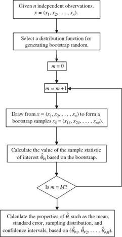
The basic algorithm of the bootstrap technique in estimating the standard deviation associated with any statistic of interest from a set of sample observations involves the following steps:
1. For a set of sample observations of size n, that is, x = {x1, x2,…, xn}, assign a probability mass 1/n to each observation according to an empirical probability distribution f,
f: P (X = xi) = 1/n for i = 1,2,…, n (6.111)
2. Randomly draw n observations from the original sample set using f to form a bootstrap sample x# = {x1#, x2#,…, xn#}. Note that the bootstrap sample x# is a subset of the original samples x.
3. Calculate the value of the sample statistic ©# of interest based on the bootstrap sample x #.
4. Independently repeat steps 2 and 3 a number of times M, obtaining bootstrap replications of в# = {в #1, в#2,…, B#M}, and calculate
|
|
|
|
|

where в#. is the average of the bootstrap replications of ©, that is,
M
в# =Y. в#m/M (6.113)
m=1
A flowchart for the basic bootstrap algorithm is shown in Fig. 6.15. The bootstrap algorithm described provides more information than just computing the
 |
standard deviation of a sample statistic. The histogram constructed on the basis of M bootstrap replications 0# = {0#i, 0#2,…, в#м} gives some ideas about the sampling distribution of the sample statistic ©, such as the failure probability. Furthermore, based on the bootstrap replications 0#, one can construct confidence intervals for the sample statistic of interest. Similar to Monte Carlo simulation, the accuracy of estimation increases as the number of bootstrap samples gets larger. However, a tradeoff exists between computational cost and the level of accuracy desired. Efron (1982) suggested that M = 200 is generally sufficient for estimating the standard errors of the sample statistics. However, to estimate the confidence interval with reasonable accuracy, one would need at least M = 1000.
This algorithm is called nonparametric, unbalanced bootstrapping. Its parametric version can be made by replacing the nonparametric estimator f by a
parametric distribution in which the distribution parameters are estimated by the maximum-likelihood method. More specifically, if one judges that on the basis of the original data set the random observations x = (x1, x2,…, xn} are from, say, a lognormal distribution, then the resampling of x’s from x using the parametric mechanism would assume that f is a lognormal distribution.
Note that the theory of the unbalanced bootstrap algorithm just described only ensures that the expected number to be resampled for each individual observation is equal to the number of bootstrap samples M generated. To improve the estimation accuracy associated with a statistical estimator of interest, Davison et al. (1986) proposed balanced bootstrap simulation, in which the number of appearances of each individual observation in the bootstrap data set must be exactly equal to the total number of bootstrap replications generated. This constrained bootstrap simulation has been found, in both theory and practical implementations, to be more efficient than the unbalanced algorithm in that the standard error associated with © by the balanced algorithm is smaller. This implies that fewer bootstrap replications are needed by the balanced algorithm than the unbalanced approach to achieve the same accuracy level in estimation. Gleason (1988) discussed several computer algorithms for implementing the balanced bootstrap simulation.
Example 6.15 Based on the annual maximum flood data listed in Table 6.4 for Miller Creek, Los Molinos, California, use the unbalanced bootstrap method to estimate the mean, standard errors, and 95 percent confidence interval associated with the annual probability that the flood magnitude exceeds 20,000 ft3/s.
Solution In this example, M = 2000 bootstrap replications of size n = 30 from {yi = ln(Xi)}, i = 1, 2,…, 30, are generated by the unbalanced nonparametric bootstrap procedure. In each replication, the bootstrapped flows are treated as lognormal
|
TABLE 6.4 Annual Maximum Floods for Mill Creek near Los Molinos, California
|
|
|
variates based on which the exceedance probability P(Q > 20,000 ft3/s) is computed. The results of the computations are shown below:
|
Statistic |
P(Q > 20,000 ft3/s) |
|
Mean |
0.0143 |
|
Coefficient of variation |
0.829 |
|
Skewness coefficient |
0.900 |
|
95 percent confidence interval |
(0.000719, 0.03722) |
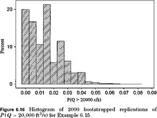
The histogram of bootstrapped replications of P (Q > 20,000 ft3/s) is shown in Fig. 6.16.
Note that the sampling distribution of the exceedance probability P (Q > 20,000 ft3/s) is highly skewed to the right. Because the exceedance probability has to be bounded between 0 and 1, density functions such that the beta distribution may be applicable. The 95 percent confidence interval shown in the table is obtained by truncating 2.5 percent from both ends of the


Leave a reply