An alternative to the graphic technique is to estimate the statistical parameters of a distribution from the sample data (refer to Sec. 3.6). Then the distribution model can be used to solve for the variate value corresponding to any desired return period or probability as
in which F-1(e) is the inverse cumulative distribution function with the model parameter vector в. Equation (3.5) can be applied when the inverse distribution function forms are analytically amenable, such as for the Gumbel, generalized extreme value, generalized logistic, and generalized Pareto distributions (see Sec. 2.6.6).
Example 3.2 Consider that the annual maximum floods follow a lognormal distribution with a mean of 490 ft3/s and a standard deviation of 80 ft3/s. Determine the flood magnitude with a 1-in-100 chance of being exceeded in any given year.
Solution From Eqs. (2.67a) and (2.67b), the parameters of a lognormal distribution, for annual maximum flood Q, can be obtained as
 Obq = ^ln (vQ +[5]) = ^ln (490) + 1 Mnq = ln(MQ) – 1 Oj2n Q = ln(490) – 1(0.1622)2 = 6.1812
Since ln( Q) follows a normal distribution with a mean of mn q = 6.1812 and a standard deviation of Oln q = 0.1622 as previously computed, the magnitude of the log – transformed 100-year flood can be calculated by
ln(g100)—= Ф-1 f 1 – -^ = Ф-1(0.99) = 2.34
Oln Q V 100 у
Hence ln(^100) = Mln Q + 2.34 x Olnq = 6.5607, and the corresponding 100-year flood magnitude can be calculated as дю0 = exp[ln(q10Q)] = 706.8 ft3/s.
For some distributions, such as Pearson type 3 or log-Pearson type 3, the appropriate probability paper or CDF inverse form is unavailable. In such a case, an analytical approach using the frequency factor KT is applied:
XT = l^x + Kt x ax (3.6)
in which xT is the variate corresponding to a return period of T, /гх and oX are the mean and standard deviation of the random variable, respectively, and KT is the frequency factor, which is a function of the return period T or P (X > xT) and higher moments, if required. It is clear that a plot of Eq. (3.6) (xT versus KT)
on linear graph paper will yield a straight line with slope of ax and intercept l^x at Kt = 0.
In order for Eq. (3.6) to be useful, the functional relationship between Kt and exceedance probability or return period must be determined for the distribution to be used. In fact, the frequency factor Kt = (xT — xx)/ax is identical to a standardized variate corresponding to the exceedance probability of 1/T for a particular distribution model under consideration. For example, if the normal distribution is considered, then Kt = zT = Ф—41 — T —:). The same applies to the lognormal distribution when the mean and standard deviation of log – transformed random variables are used. Hence the standard normal probability table (Table 2.2) provides values of the frequency factor for sample data from normal and log normal distributions. Once this relation is known, a nonlinear probability or return-period scale can be constructed to replace the linear Kt scale, and thus special graph paper can be constructed for any distribution so that plot of xT versus P or T will be linear.
Gumbel probability paper has been printed, although it is not readily available from commercial sources. Referring to Eq. (2.85a), the relationship between Kt and T for this distribution can be derived as


For Pearson and log-Pearson type 3 distributions, linearization can be accomplished according to Eq. (3.6). However, for this distribution, the frequency factor is a function of both P or T and the skewness coefficient yx. This means that a different nonlinear P or T scale is required for each skewness coefficient, and therefore, it is impractical to construct a probability paper for this distribution. However, it should be pointed out that if yx = 0 in log-space, the log-Pearson type 3 reduces to the lognormal distribution, and thus commercial lognormal probability paper can be used. The relationship between frequency factor Kt, T, and yx cannot be developed in a closed form, as was done for the Gumbel distribution in Eq. (3.7). However, the relationship can be computed numerically, and the results are given in Table 3.3. For 0.99-1 < T < 100 and |yx | < 2, the frequency-factor values are well approximated by the Wilson – Hilferty transformation (Stedinger et al., 1993):
in which zT is the standard normal quantile with exceedance probability of 1/T.
The procedure for using the frequency-factor method is outlined as follows: 1
|
Return period in years
|
Skewness coefficient yx
|
2
|
5
|
10 25 50 Exceedence probability
|
100
|
200
|
|
0.50
|
0.20
|
0.10
|
0.04
|
0.02
|
0.01
|
0.005
|
|
3.0
|
-0.396
|
0.420
|
1.180
|
2.278
|
3.152
|
4.051
|
4.970
|
|
2.9
|
-0.390
|
0.440
|
1.195
|
2.277
|
3.134
|
4.013
|
4.909
|
|
2.8
|
-0.384
|
0.460
|
1.210
|
2.275
|
3.114
|
3.973
|
4.847
|
|
2.7
|
-0.376
|
0.479
|
1.224
|
2.272
|
3.093
|
3.932
|
4.783
|
|
2.6
|
-0.368
|
0.499
|
1.238
|
2.267
|
3.071
|
3.889
|
4.718
|
|
2.5
|
-0.360
|
0.518
|
1.250
|
2.262
|
3.048
|
3.845
|
4.652
|
|
2.4
|
-0.351
|
0.537
|
1.262
|
2.256
|
3.023
|
3.800
|
4.584
|
|
2.3
|
-0.341
|
0.555
|
1.274
|
2.248
|
2.997
|
3.753
|
4.515
|
|
2.2
|
-0.330
|
0.574
|
1.284
|
2.240
|
2.970
|
3.705
|
4.444
|
|
2.1
|
-0.319
|
0.592
|
1.294
|
2.230
|
2.942
|
3.656
|
4.372
|
|
2.0
|
-0.307
|
0.609
|
1.302
|
2.219
|
2.912
|
3.605
|
4.298
|
|
1.9
|
-0.294
|
0.627
|
1.310
|
2.207
|
2.881
|
3.553
|
4.223
|
|
1.8
|
-0.282
|
0.643
|
1.318
|
2.193
|
2.848
|
3.499
|
4.147
|
|
1.7
|
-0.268
|
0.660
|
1.324
|
2.179
|
2.815
|
3.444
|
4.069
|
|
1.6
|
-0.254
|
0.675
|
1.329
|
2.163
|
2.780
|
3.388
|
3.990
|
|
1.5
|
-0.240
|
0.690
|
1.333
|
2.146
|
2.743
|
3.330
|
3.910
|
|
1.4
|
-0.225
|
0.705
|
1.337
|
2.128
|
2.706
|
3.271
|
3.828
|
|
1.3
|
-0.210
|
0.719
|
1.339
|
2.108
|
2.666
|
3.211
|
3.745
|
|
1.2
|
-0.195
|
0.732
|
1.340
|
2.087
|
2.626
|
3.149
|
3.661
|
|
1.1
|
-0.180
|
0.745
|
1.341
|
2.066
|
2.585
|
3.087
|
3.575
|
|
1.0
|
-0.164
|
0.758
|
1.340
|
2.043
|
2.542
|
3.022
|
3.489
|
|
0.9
|
-0.148
|
0.769
|
1.339
|
2.018
|
2.498
|
2.957
|
3.401
|
|
0.8
|
-0.132
|
0.780
|
1.336
|
1.993
|
2.453
|
2.891
|
3.312
|
|
0.7
|
-0.116
|
0.790
|
1.333
|
1.967
|
2.407
|
2.824
|
3.223
|
|
0.6
|
-0.099
|
0.800
|
1.328
|
1.939
|
2.359
|
2.755
|
3.132
|
|
0.5
|
-0.083
|
0.808
|
1.323
|
1.910
|
2.311
|
2.686
|
3.041
|
|
0.4
|
-0.066
|
0.816
|
1.317
|
1.880
|
2.261
|
2.615
|
2.949
|
|
0.3
|
-0.050
|
0.824
|
1.309
|
1.849
|
2.211
|
2.544
|
2.856
|
|
0.2
|
-0.033
|
0.830
|
1.301
|
1.818
|
2.159
|
2.472
|
2.763
|
|
0.1
|
-0.017
|
0.836
|
1.292
|
1.785
|
2.107
|
2.400
|
2.670
|
|
0.0
|
0
|
0.842
|
1.282
|
1.751
|
2.054
|
2.326
|
2.576
|
|
-0.1
|
0.017
|
0.846
|
1.270
|
1.716
|
2.000
|
2.252
|
2.482
|
|
-0.2
|
0.033
|
0.850
|
1.258
|
1.680
|
1.945
|
2.178
|
2.388
|
|
-0.3
|
0.050
|
0.853
|
1.245
|
1.643
|
1.890
|
2.104
|
2.294
|
|
-0.4
|
0.066
|
0.855
|
1.231
|
1.606
|
1.834
|
2.029
|
2.201
|
|
-0.5
|
0.083
|
0.856
|
1.216
|
1.567
|
1.777
|
1.955
|
2.108
|
|
-0.6
|
0.099
|
0.857
|
1.200
|
1.528
|
1.720
|
1.880
|
2.016
|
|
-0.7
|
0.116
|
0.857
|
1.183
|
1.488
|
1.663
|
1.806
|
1.926
|
|
-0.8
|
0.132
|
0.856
|
1.166
|
1.448
|
1.606
|
1.733
|
1.837
|
|
-0.9
|
0.148
|
0.854
|
1.147
|
1.407
|
1.549
|
1.660
|
1.749
|
|
-1.0
|
0.164
|
0.852
|
1.128
|
1.366
|
1.492
|
1.588
|
1.664
|
|
-1.1
|
0.180
|
0.848
|
1.107
|
1.324
|
1.435
|
1.518
|
1.581
|
|
-1.2
|
0.195
|
0.844
|
1.086
|
1.282
|
1.379
|
1.449
|
1.501
|
|
-1.3
|
0.210
|
0.838
|
1.064
|
1.240
|
1.324
|
1.383
|
1.424
|
|
-1.4
|
0.225
|
0.832
|
1.041
|
1.198
|
1.270
|
1.318
|
1.351
|
|
-1.5
|
0.240
|
0.825
|
1.018
|
1.157
|
1.217
|
1.256
|
1.282
|
|
-1.6
|
0.254
|
0.817
|
0.994
|
1.116
|
1.166
|
1.197
|
1.216
|
|
|
Return period in years
|
Skewness coefficient yx
|
2
|
5
|
10 25 50 Exceedence probability
|
100
|
200
|
|
0.50
|
0.20
|
0.10
|
0.04
|
0.02
|
0.01
|
0.005
|
|
-1.7
|
0.268
|
0.808
|
0.970
|
1.075
|
1.116
|
1.140
|
1.155
|
|
-1.8
|
0.282
|
0.799
|
0.945
|
1.035
|
1.069
|
1.087
|
1.097
|
|
-1.9
|
0.294
|
0.788
|
0.920
|
0.996
|
1.023
|
1.037
|
1.044
|
|
-2.0
|
0.307
|
0.777
|
0.895
|
0.959
|
0.980
|
0.990
|
0.995
|
|
-2.1
|
0.319
|
0.765
|
0.869
|
0.923
|
0.939
|
0.946
|
0.949
|
|
-2.2
|
0.330
|
0.752
|
0.844
|
0.888
|
0.900
|
0.905
|
0.907
|
|
-2.3
|
0.341
|
0.739
|
0.819
|
0.855
|
0.864
|
0.867
|
0.869
|
|
-2.4
|
0.351
|
0.725
|
0.795
|
0.823
|
0.830
|
0.832
|
0.833
|
|
-2.5
|
0.360
|
0.711
|
0.771
|
0.793
|
0.798
|
0.799
|
0.800
|
|
-2.6
|
0.368
|
0.696
|
0.747
|
0.764
|
0.768
|
0.769
|
0.769
|
|
-2.7
|
0.376
|
0.681
|
0.724
|
0.738
|
0.740
|
0.740
|
0.741
|
|
-2.8
|
0.384
|
0.666
|
0.702
|
0.712
|
0.714
|
0.714
|
0.714
|
|
-2.9
|
0.390
|
0.651
|
0.681
|
0.683
|
0.689
|
0.690
|
0.690
|
|
-3.0
|
0.396
|
0.636
|
0.666
|
0.666
|
0.666
|
0.667
|
0.667
|
SOURCE: U. S. Water Resources Council (1981).
|
2. For the desired return period, determine the associated value of KT for the distribution.
3. Compute the desired quantile value using Eq. (3.6) with x replacing цx and sx replacing ax, that is,
XT = x + KT x sx (3.9)
It should be recognized that the basic difference between the graphic and analytical approaches is that each represents a different method of estimating the statistical parameters of the distribution being used. By the analytical approach, a best-fit line is constructed that then sets the statistical parameters. In the mathematical approach, the statistical parameters are first computed from the sample, and effectively, the line thus determined is used. The line determined using the mathematical approach is in general a poorer fit to the observed data than that obtained using the graphic approach, especially if curve-fitting procedures are applied. However, the U. S. Water Resources Council (1967) recommended use of the mathematical approach because
1. Graphic least-squares methods are avoided to reduce the incorporation of the random characteristics of the particular data set (especially in the light of the difficulty in selecting the proper plotting-position formula).
2. The generally larger variance of the mathematical approach is believed to help compensate for the typically small data sets.
Example 3.3 Using the frequency-factor method, estimate the flows with return periods of 2, 10, 25, 50, and 100 years for the Boneyard Creek using the Gumbel and log-Pearson type 3 distributions. Use the historical data in Example 3.1 as a basis for the calculations.
Solution Based on the samples, the method requires determination of the frequency factor Kt in
xt = x + Kt x sx
For the Gumbel distribution, values of Kt can be calculated by Eq. (3.7). For the log-Pearson type 3 distribution, Table 3.3 or Eq. (3.8) can be used, which requires computation of the skewness coefficient. The calculations of relevant sample moments are shown in the following table:
|
Year
|
|
Original scale
|
Log – Transformed scale
|
|
gi (ft3/s)
|
gi2
|
gi3
|
Уі = ln( gi)
|
Уі2
|
Уі3
|
|
1961
|
390
|
1.52e + 05
|
5.93e + 07
|
5.97
|
35.59
|
212.36
|
|
1962
|
374
|
1.40e + 05
|
5.23e + 07
|
5.92
|
35.10
|
207.92
|
|
1963
|
342
|
1.17e + 05
|
4.00e + 07
|
5.83
|
34.05
|
198.65
|
|
1964
|
507
|
2.57e + 05
|
1.30e + 08
|
6.23
|
38.79
|
241.63
|
|
1965
|
596
|
3.55e + 05
|
2.12e + 08
|
6.39
|
40.84
|
260.95
|
|
1966
|
416
|
1.73e + 05
|
7.20e + 07
|
6.03
|
36.37
|
219.33
|
|
1967
|
533
|
2.84e + 05
|
1.51e + 08
|
6.28
|
39.42
|
247.50
|
|
1968
|
505
|
2.55e + 05
|
1.29e + 08
|
6.22
|
38.75
|
241.17
|
|
1969
|
549
|
3.01e + 05
|
1.65e + 08
|
6.31
|
39.79
|
251.01
|
|
1970
|
414
|
1.71e + 05
|
7.10e + 07
|
6.03
|
36.31
|
218.81
|
|
1971
|
524
|
2.75e + 05
|
1.44e + 08
|
6.26
|
39.21
|
245.49
|
|
1972
|
505
|
2.55e + 05
|
1.29e + 08
|
6.22
|
38.75
|
241.17
|
|
1973
|
447
|
2.00e + 05
|
8.93e + 07
|
6.10
|
37.24
|
227.27
|
|
1974
|
543
|
2.95e + 05
|
1.60e + 08
|
6.30
|
39.65
|
249.70
|
|
1975
|
591
|
3.49e + 05
|
2.06e + 08
|
6.38
|
40.73
|
259.92
|
|
Sum =
|
7236
|
3.58e + 06
|
1.81e + 09
|
92.48
|
570.58
|
3522.88
|
|
For the Gumbel distribution,
|
For the log-Pearson type 3 distribution,
|
|
|
|
|
У =
|
n
|
15
|
|
sy =
|
1—1 1
1 1
|
|
gy =
|
n
|
m3
|
|
(n – 1)(n – 2) syj
|
|
|
|
|
|
15(-0.00336) (14)(13)(0.173)3
|
|
|
|
|
in which m3 = Уз — Уі + 2ny3. The determination of the values of frequency
factor corresponding to different return periods is shown in the following table:
Frequency factor by distribution
|
Return period
|
Exceedance
|
Nonexceedance
|
Gumbel
|
LP3
|
|
(years)
|
probability
|
probability
|
Eq. (3.7)
|
Eq. (3.8)
|
|
2
|
0.50
|
0.50
|
—0.1643
|
0.0892
|
|
10
|
0.10
|
0.90
|
1.3046
|
1.2093
|
|
25
|
0.04
|
0.96
|
2.0438
|
1.5526
|
|
50
|
0.02
|
0.98
|
2.5923
|
1.7570
|
|
100
|
0.01
|
0.99
|
3.1367
|
1.9292
|
|
Based on the preceding frequency-factor values, the flood magnitude of the various
|
|
return periods
|
can be determined as
|
|
|
|
|
Frequency curves
|
by distribution (ft3/s)
|
|
Return period
|
|
Gumbel
|
|
LP3
|
|
(years)
|
qT = 482.4 + 79.8Kt, EV1
|
qT = exp(6.165 + 0.173Kt, LP3)
|
|
2
|
|
469.3
|
|
483.3
|
|
10
|
|
586.5
|
|
586.4
|
|
25
|
|
645.4
|
|
622.2
|
|
50
|
|
689.2
|
|
644.5
|
|
100
|
|
732.6
|
|
663.9
|
One could compare these results for the Gumbel distribution with those obtained from the graphic approach of Example 3.1.
|
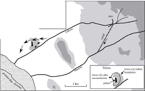
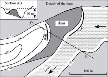
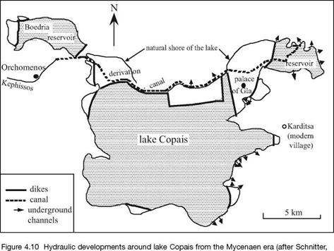
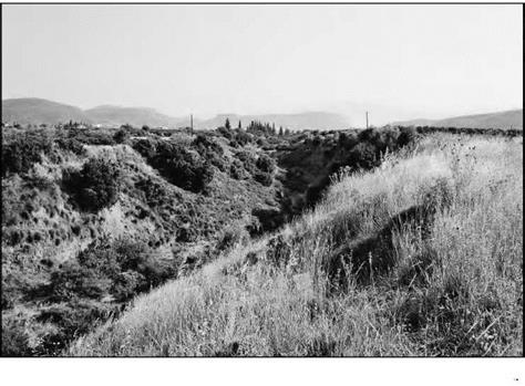 Figure 4.14 Lakissa diversion canal, looking from the top of the Kofini dam (photo by the author)



![STEP 6 RAISE THE WALLS Подпись: 1. To mark the cut line, position the brace diagonally across the wall section from the bottom plate to the double top plate, and then pencil a line along one edge of every framing member the brace crosses. [Photo © Larry Haun]](/img/1312/image329_0.gif)

![STEP 6 RAISE THE WALLS Подпись: The first wall goes up! Make sure you have enough help when you're ready to raise the walls. Have one person take charge, and get everyone to lift in unison. [Photo by HFHI/Will Crocker]](/img/1312/image331_0.gif) When you remove the temporary blocks nailed to the rim joist, be sure to pull the nails or bend them over so that no one gets a nail in the foot!
When you remove the temporary blocks nailed to the rim joist, be sure to pull the nails or bend them over so that no one gets a nail in the foot!


 used to cut 2x stock with a handsaw and nail them between the studs, running it diagonally from plate to plate. It was a good brace, but it took about an hour to make each one. These days, braces are much easier to install. You can attach L-shaped metal angle braces or nail plywood or OSB sheathing to the frame. Code requirements vary, so be sure to check with your building department to find out how the walls should be braced. In some areas, bracing is also required on certain interior walls.

