Summary and Conclusions
Hwang et al. (1981) presented a review of literature related to system reliability evaluation techniques for small to large complex systems. A large system was defined as one that has more than 10 components and a moderate system as one which has more than 6 components and less than 10. Complex systems were defined as ones that could not be reduced to a series-parallel system. Hwang et al. concluded that for a large, complex system, computer programs should be used that provide the minimum cut sets and calculate the minimal cut approximation to system reliability. Minimal paths can be generated from minimum cuts. Based on minimum cut sets, reliability approximations then can be obtained for large, complex networks. Hwang et al. also noted that Monte Carlo methods for system reliability evaluation can be used when component reliabilities are sampled by the Monte Carlo method. They also identified several miscellaneous approaches for evaluating complex systems, including a moment method, a block-diagram method, Bayesian decomposition, and decomposition by Boolean expression.
Hwang et al. (1981) concluded that of all the evaluation techniques in the papers surveyed, only a few had limited success in solving some large, complex
system reliability problems, and few techniques have been completely effective when applied to large system reliability problems. They suggested that a generally efficient graph partitioning technique for reliability evaluation of large, highly interconnected networks should be developed.
Since the 1981 paper by Hwang et al., several other system reliability evaluation techniques have been reported in the literature. Aggarwal et al. (1982) presented a method that uses decomposition of a probabilistic graph using cut sets. The method is applied to a simplified network with five nodes and seven links, and only limited computational results are presented.
Appendix 7A: Derivation of Bounds for Bivariate Normal Probability
Consider two performance functions Wj (Z’) = 0 and Wm(Z’) = 0 in a twodimensional standardized, uncorrelated normal space whose design points are z j * and z m*, respectively. At each of the design points, the first-order failure hyperplanes can be expressed as
Wj (Zо = 0 ^ (Z – 4, j*) = aj + ayZ[ + ayZ2 (7A.1)
k=1 ‘ k ‘
2 f d W
Wm(Z0 = 0 ^ ^ 4 rrj, ) (Zk — Zk m*) = a0m + a1mZ1 + a2mZ2 (7A.2)
іґЛd Zkl,
in which zk, m* is the coordinate of the kth stochastic basic variable at the design point z’m* of the mth performance function, and
The covariance between the two performance functions can be obtained as
Cov[Wj (Z/), Wm(Z )] = E{[(a0j + a1jZ1 + a2jZ2) — a0j]
x [(a0m + a1mZ1 + a2mZ2) — a0m]}
= E [(a1jZ1 + a2jZ2)(a1mZ1 + a2mZ2)]
= a1ja1m + a2ja2m (7A..3)
Hence the correlation coefficient between the two performance functions at the design points is

|
|
|
|
|
|
|
|
|
This can be generalized to multidimensional problems involving M stochastic basic variables as
Note that the preceding correlation coefficient between the two performance functions Pjm is exactly equal to the inner product of the corresponding directional derivative vectors
— ![]() ( aj*) ( am*) — (aj*) (am*)
( aj*) ( am*) — (aj*) (am*)
— |aj||am*| cos в
— cos в
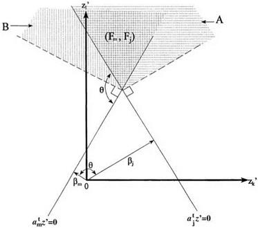
in which в is the angle between the directional derivatives of the two performance functions. Hence, if the two performance functions are positively correlated, the angle в between am* and aj * lies in the range 0° < в < 90°. On the other hand, negative correlation between Wj (Z) and Wm(Z) corresponds to the range 90° < в < 180°. Plots for positively and negatively correlated performance functions are show in Figs. 7A.1 and 7A.2, respectively.
When Wj (Z) and Wm(Z) are positively correlated, that is, pjm > 0, referring to Fig. 7A.1, the shaded area representing the joint failure of the two performance functions satisfies the following relationships:
(Fj, Fm) э A and (Fj, Fm) э B
in which (Fj, Fm) represents the joint failure events of the two performance functions, and sets A and B are defined in Fig. 7A.1.
Again, referring to Fig. 7A.1, the following relationship holds:
Max[P(A), P (B)] < P(Fj, Fm) < P(A) + P (B) (7A.7)
By orthogonality, one has
P (A) — Ф(-Pm)Ф(Pj | m) (7A.8)
P (B) — Ф(вj m, Pmj) (7A.9)
1 n ej — pjmfim „ Pm — pmjPj. л лл
where Pj | m — , =- Pm | j — , = (7A.10)
V 1 — Pjm у 1 — pmj
which are defined in Fig. 7A.1.
|
|
|
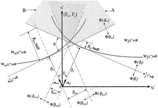
Referring to Fig. 7A.2 for negatively correlated Wj (Z) and Wm(Z), it can be observed that
(Fj, Fm) c A and (Fj, Fm) c B
resulting in
0 < P(Fj, Fm) < min[P(A), P(B)] (7A.11)

with P(A) and P(B) given in Eqs.(7A.8) and (7A.9), respectively.
7.1
 |
|
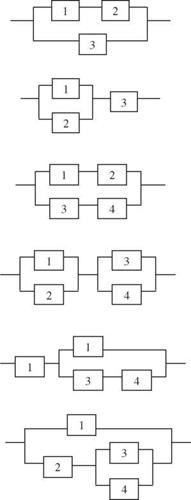
Derive the expression of system reliability for the system configurations shown in Fig. 7P.1 under the condition of (a) all units are dependent and different and (b) all units are independent and identical.
7.2 Consider that two independent, identical units are to be added to an existing unit that would result in three units in the whole system.
(a) Sketch all possible system configurations according to the arrangement of the three units.
(b) Rank your system configurations according to the system reliability.
7.3 Consider the two system configurations shown in Fig. 7P.2. Use the cut-set method to determine the system reliability. Assume that all system components are identical and behave independently of each other.
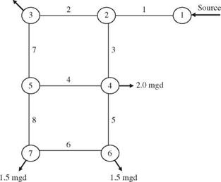
7.4 Consider a hypothetical water distribution network consisting of two loops, as shown in Fig. 7P.3. Let’s say that the service failure of the system is when at least one demand node cannot receive water. (a) Construct a tree diagram indicating failure cases for the water distribution network. (b) Determine the system reliability if all pipe sections behave independently, and each has a breakage probability of 0.03.
7.5 Resolve Problem 7.4 by cut-set analysis.
7.6 Resolve Problem 7.4 by tie-set analysis
7.7 Resolve Problem 7.4 by the conditional probability approach.
7.8 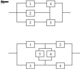
A detention basin is designed to accommodate excessive surface runoff temporarily during storm events. The detention basin should not overflow, if possible, to prevent potential pollution of the stream or other receiving water bodies. For simplicity, the amount of daily rainfall is categorized as heavy, moderate, and light (including none). With the present storage capacity, the detention basin is capable of accommodating runoff generated by two consecutive days of heavy rainfall or three consecutive days of at least moderate rainfall. The daily rainfall amounts around the detention basin site are not entirely independent. In other
|
|
|
2.5 mgd |
|
Figure 7.3 Hypothetical water distribution network. |
words, the amount of daily rainfall on a given day would affect the daily rainfall amount on the next day. Let random variable Xt represent the amount of rainfall on any day t. The transition probability matrix, indicating the conditional probability of rainfall amount in a given day t conditioned on the rainfall amount of the previous day t — 1, is shown in the following table (after Mays and Tung 1992).
|
Xt+1 |
|||
|
Heavy (H) |
Moderate (M) |
Light (L) |
|
|
X t Heavy (H) |
0.3 |
0.5 |
0.2 |
|
Moderate (M) |
0.3 |
0.4 |
0.3 |
|
Light (L) |
0.1 |
0.3 |
0.6 |


Leave a reply