The basic functions of highway drainage structures are (1) as hydraulic facilities to safely convey floods under highways during all but the most severe flooding conditions and (2) as portions of the highway to move highway traffic freely over stream channels. There are three general types of drainage structures: bridges, box culverts, and pipe culverts. Conventionally, bridges refer to structures measuring more than 20 ft along the roadway centerline (AASHTO, 1979). Box culverts are usually built of concrete with rectangular openings. Pipe culverts can be in various geometric forms, such as circular, arch, etc., and can be made of several different materials, such as steel, cast iron, concrete, or plastic.
The design of highway drainage structures involves both hydraulic design and structural design. The discharge associated with the critical flood that starts to cause hazards to life, property, and stream stability is termed as the hydraulic design discharge. The process to select the design discharge and to perform the necessary hydraulic computations for a proposed highway structure is called hydraulic design. In practice, the design discharge is one-to-one related to the design frequency through frequency analysis. Therefore, the design event also can be characterized by the design frequency. In this example, the design frequency refers to an annual exceedance probability or its reciprocal, the design return period.
The example problem under consideration is to design a circular culvert under a two-lane highway. The culvert is 100 ft long. The equivalent average daily traffic is 3000 vehicles per day. The discount rate used is 7.125 percent, and the useful service life of the culvert structure is estimated to be 35 years. Detailed descriptions of this example are given by Tung and Bao (1990).
In this example, only the inherent hydrologic and parameter uncertainties are considered. The primary objectives are (1) to search for the optimal design parameters associated with the minimum total annual expected cost for the culvert and (2) to investigate the sensitivity of the optimal design parameters with respect to (a) the hydrologic parameter uncertainty, (b) the length of streamflow records, (c) the distribution model of flood flow, and (d) the maximum flood-damage cost. More specifically, the optimal design parameters considered in this example are the optimal design return period T and the associated least total annual expected cost (LTAEC).
The estimated sample mean and sample standard deviation for the flood flow are 47.9 and 71.9 ft3/s, respectively. The skewness coefficient of streamflow for the original scale and log-transformed scale are assumed to be 0.5 and 0.2, respectively.
In the sensitivity analysis, the optimal total annual expected cost was calculated for various record lengths n of 10, 20, 40, 60, and 100 years; for maximum
flood damage cost Dmax of $928, $1500, $3500, and $4500; and for flood flow distribution models of normal, lognormal, Pearson type 3, and log-Pearson type 3 probability distributions.
The cost function representing the annual installation (first) cost of the culvert is derived on the basis of data from Corry et al. (1980) using regression analysis:
AFC = 1.0215 – 2.62 x 10⁻⁷qc2 (8.38)
where AFC is the annual first cost ($), and qc is the design discharge (ft3/s). The R2 of this regression equation is 0.976.
The damage function D(q), approximating the original discrete form in Corry et al. (1980) by a continuous function, can be expressed as
 q ^ qmax

 qc < q < qmax (8.39)
q < qc
where Dmax is the maximum flood damage cost, qmax is the flood magnitude corresponding to Dmax, and qc is the design discharge. It is understood that, in general, qmax will be increased as a result of raising the design discharge qc. The rate ofincrease in qmax will slow down as qc increases. The damage function used, for illustration, is shown in Fig. 8.13, in which qmax is determined from
qmax = 210 + qc – q094 (8.40)

|
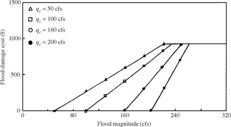
Figure 8.13 Flood-damage function in risk-based culvert design example.
|
|
Because of the complexity of the functional form of the objective function, it is difficult to solve Eqs. (8.31) and (8.33) analytically. Therefore, optimum search techniques are useful to solve the problem. However, gradient search techniques are inappropriate for use in this case because the gradient of the objective function is not easily computable. Among the search techniques that do not require knowledge of gradient of the objective function, Fibonacci search is an efficient technique to be used for this single-decision variable-optimization problem (Sivazlian and Stanfel, 1974).
Fibonacci search applies the sequential search strategy that successively reduces the feasible decision variable interval to 1/FN its original size with just N function evaluations. The final decision-variable interval can be made as close to the optimal solution as the desired accuracy. FN is called the N th Fibonacci number in the Fibonacci sequence FN, for i = 0, 1, 2, 3,…, whose value is given by the recurrence relation
 F0 = F1 = 1
Fi+1 = Ft + Fi-1 i > 1
The computational procedures for determination of the optimal return period corresponding to the optimal capacity in the risk-based design of a pipe culvert considering the hydrologic inherent and parameter uncertainties is illustrated in Fig. 8.14.
The optimal design frequency T * and the associated LTAEC under different record lengths n and streamflow probability distributions with maximum flood damage cost (Dmax = $928) are listed in Table 8.3. The values in the columns for n = 10-100 are calculated by considering hydrologic parameter uncertainty, whereas the values in the column with n =<x were calculated without considering hydrologic parameter uncertainty.
Comparing the two design methods, the value of the LTAEC without considering parameter uncertainty is always smaller than the value considering parameter uncertainty regardless of the probability distributions or values of Dmax. This observation shows that neglect of the hydrologic parameter uncertainty could lead to an underestimation of the total expected cost.
The value of LTAEC decreases as the record length increases. This is expected because the effect of hydrologic parameter uncertainty involved in estimating the second cost diminishes as the record length for streamflow gets longer. The difference in LTAEC values calculated by the two methods, for Dmax = $928 and n > 20, is only about 3 percent for any of the four probability distributions considered. However, the higher the value of Dmax, the more dominant the second cost becomes in the objective function evaluation. Therefore, the difference in LTAEC values by the two methods at the same record length will be larger as Dmax is increased.
Examining the T * values in Table 8.3, the difference in T * between the two methods is less than 20 percent in most cases. Also, for fixed distribution and sample size, the optimal T * increases as Dmax increases (see Table 8.4).
|
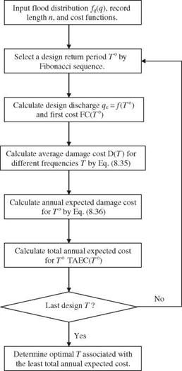
Figure 8.14 Flowchart of optimal risk-based design of a pipe culvert.
|
This confirms the original intuition. However, there does not exist the same consistent tendency in T * as with the LTAEC shown earlier. Therefore, when T * is considered as a criterion in the comparison of the two design methods, it is difficult to conclude which method tends to be more conservative.
Figure 8.15 shows of the total annual expected cost function, annual first-cost function, and annual second-cost function versus the design return period T with record length varying from 10 to 100 years at -Dmax = $4500 for the lognormal probability distribution. Similar behavior was observed for three other
|
TABLE 8.3 Optimal Design Return Period T and LTAEC for Different Distributions and Record Lengths When Dmax = $928
|
Flood distribution
|
Optimal
design
|
|
Record length (in years)
|
|
|
10
|
20
|
40
|
60
|
100
|
|
|
Normal
|
T * (years)
|
4.82
|
4.62
|
4.55
|
4.55
|
4.20
|
4.00
|
|
LTAEC ($)
|
473.5
|
461.7
|
456.2
|
454.7
|
453.5
|
448.1
|
|
Lognormal
|
T * (years)
|
5.79
|
6.00
|
6.27
|
6.55
|
6.20
|
6.96
|
|
LTAEC ($)
|
446.7
|
433.9
|
428.1
|
425.9
|
423.2
|
420.2
|
|
Pearson type 3
|
T * (years)
|
4.52
|
4.62
|
4.55
|
4.55
|
4.55
|
4.00
|
|
LTAEC ($)
|
479.9
|
468.3
|
462.6
|
461.0
|
459.8
|
454.1
|
|
Log-Pearson type 3
|
T * (years)
|
5.79
|
6.00
|
6.20
|
6.41
|
6.13
|
6.68
|
|
LTAEC ($)
|
450.5
|
438.0
|
432.3
|
430.2
|
427.4
|
424.6
|
SOURCE: After Tung and Bao (1990).
|
types of distributions. From Fig. 8.15 it is clear that the annual second cost (ASC) and the total annual expected cost (TAEC) decrease as the record length increases. Therefore, the LTAEC will be smaller when the record length gets longer. However, the corresponding T *, as discussed earlier, may not necessarily
Record length (in years)
|
TABLE 8.4 List of Optimal Design Return Period (7*) Under Different Record Lengths, Flood Distributions, and Maximum Flood Damage
Flood
|
Dmax
|
distribution
|
10
|
20
|
40
|
60
|
100
|
|
|
$928
|
N
|
4.82
|
4.62
|
4.55
|
4.55
|
4.20
|
4.00
|
|
LN
|
5.79
|
6.00
|
6.27
|
6.55
|
6.20
|
6.96
|
|
P3
|
4.62
|
4.62
|
4.55
|
4.55
|
4.55
|
4.00
|
|
LP3
|
5.79
|
6.00
|
6.20
|
6.41
|
6.13
|
6.68
|
|
$1500
|
N
|
6.62
|
6.75
|
6.37
|
7.03
|
6.68
|
6.96
|
|
LN
|
7.51
|
7.99
|
7.99
|
7.79
|
7.58
|
7.03
|
|
P3
|
6.41
|
6.62
|
7.03
|
6.75
|
6.48
|
6.96
|
|
LP3
|
7.37
|
6.68
|
7.86
|
7.51
|
7.03
|
7.03
|
|
$2500
|
N
|
10.47
|
8.13
|
9.51
|
8.48
|
8.75
|
9.17
|
|
LN
|
10.41
|
10.61
|
10.06
|
9.44
|
9.30
|
10.96
|
|
P3
|
9.17
|
9.72
|
8.89
|
8.13
|
7.79
|
7.03
|
|
LP3
|
9.85
|
9.92
|
9.51
|
9.44
|
8.75
|
10.34
|
|
$3500
|
N
|
13.51
|
12.75
|
12.89
|
13.30
|
12.54
|
11.03
|
|
LN
|
12.27
|
12.27
|
11.37
|
11.65
|
12.13
|
11.03
|
|
P3
|
11.71
|
11.65
|
11.16
|
11.44
|
11.37
|
11.03
|
|
LP3
|
11.51
|
11.58
|
11.30
|
11.44
|
11.65
|
11.03
|
|
$4500
|
N
|
17.98
|
17.71
|
16.26
|
14.75
|
15.71
|
12.89
|
|
LN
|
14.61
|
13.92
|
13.85
|
13.92
|
13.64
|
11.03
|
|
P3
|
14.26
|
13.78
|
13.92
|
13.85
|
12.68
|
11.03
|
|
LP3
|
13.57
|
13.09
|
13.37
|
13.02
|
12.61
|
11.03
|
NOTE: N = normal; LN = lognormal; P3 = Pearson type 3; LP3 = log-Pearson type 3 SOURCE: After Tung and Bao (1990).
|
|
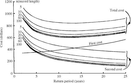
Figure 8.15 Total annual expected costs in optimal risk-based design of pipe culvert with various record lengths under lognormal distribution. (After Tung and Bao, 1990.)
|
become smaller as the record length increases. The inconsistent behavior between T * and LTAEC in comparing the two design methods is mainly attributed to the nonlinear and nonmonotonic relationship between T * and LTAEC.
It can be seen from Fig. 8.15 that the total annual expected cost (TAEC) curves are very flat in a range of design frequencies from 5 to 20 years for this example. Therefore, from a practical point of view, a pipe culvert could be overdesigned about 5 to 10 years above the optimal design frequency to give more confidence in the safety protection of the structure with only a small fraction of extra annual capital investment.


 Coconut palm flooring, like bamboo, is plentiful and can be sustainably harvested. Its texture is fine pored, reminiscent of mahogany. Because coconut palm is a dark wood, its color range is limited, from a rich, mahogany red to a deep brown. And it is tough stuff: Smith & Fong™ offers a %-in.-thick, three-ply, tongue-and-groove strip flooring, called Durapalm®, which it claims to be 25 percent harder than red oak. Durapalm is available unfinished or prefinished. One of the finish options contains space-age ceramic particles for an even tougher surface. So if you’re thinking of installing a ballroom floor in your bungalow, this is definitely a material to consider.

 Developed and first adopted in Europe, laminate flooring is most commonly snap-together planks that float above a substrate, speeding installation, repairs, and removal. Of all flooring materials, laminate is probably the most affordable; and as noted, it’s almost indestructible. Because it resists scratches, chemicals, burns, and water, it’s a good choice for high-use or high – moisture areas. It’s also colorfast, dimensionally stable, and easy to clean—though many manufacturers insist that you use proprietary cleaning solutions. For a good overview of installing laminates, see
  bed. Trench fields depend on separation to work properly. To expand on this, let me give you some technical information.
 If you are faced with hilly land to work with, a trench system is ideal. The trenches can be dug to follow the contour of the land. This gives you maximum utilization of the sloping ground.
 qc < q < qmax (8.39)


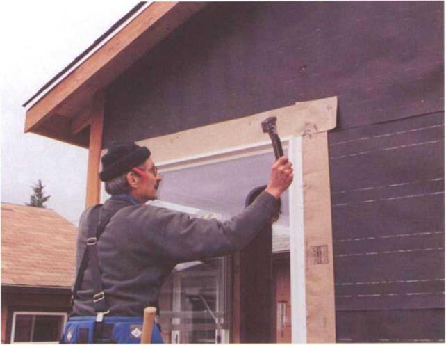
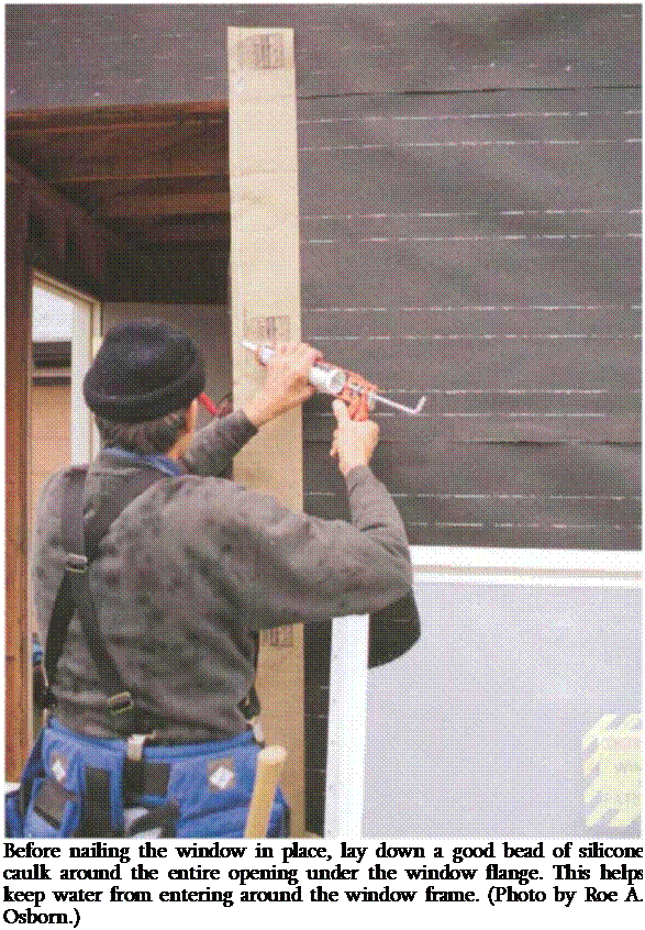 erly and don’t allow moisture or air to penetrate the building envelope. Let’s start with windows.





![Install the baseboard trim Подпись: INSIDE BASEBOARD CORNERS ARE COPED. The coped cut fits the profile of the trim piece that runs into the corner. [Photo * The Taunton Press, Inc.]](/img/1312/image956.gif) The second piece of baseboard is coped to fit against the first piece and cut square to butt against the next wall. On the end that will mate with the short piece of baseboard, cut a 45-degree miter that is long on the back (so you can see the cut surface). Now use a coping saw to cut the outline of the profile left in the exposed end grain (see the sidebar on the facing page). The cope-cut end will fit snugly against the first piece of baseboard (see the photo below).
The second piece of baseboard is coped to fit against the first piece and cut square to butt against the next wall. On the end that will mate with the short piece of baseboard, cut a 45-degree miter that is long on the back (so you can see the cut surface). Now use a coping saw to cut the outline of the profile left in the exposed end grain (see the sidebar on the facing page). The cope-cut end will fit snugly against the first piece of baseboard (see the photo below).